Customising Plots

Plotting the cumulative distribution

The ssdtools package produces a plot of the cumulative distribution functions for the multiple input distributions through the use of the ssd_plot_cdf() function. For example, consider the boron data. We can fit, and then plot the cdf using:

library(ggplot2)
library(ssdtools)

fits <- ssd_fit_dists(ssddata::ccme_boron)
gp <- ssd_plot_cdf(fits)

print(gp)

This graphic is a ggplot object and so can be saved and embellished in the usual way.

Customising the cumulative distribution plot

Plot the model-averaged fit with individual fits

We can add the model-averaged cdf by first obtaining predicted values, and extending the default ssdtools ggplot in the usual way using geom_line:

library(ssddata)
library(ssdtools)
library(ggplot2)

dist <- ssdtools::ssd_fit_dists(ssddata::ccme_boron)
pred <- predict(dist, ci = FALSE)
boron_hc5 <- ssd_hc(dist)
ssdtools::ssd_plot_cdf(dist) +
  geom_line(data = pred, aes(x = est, y = proportion, colour = "Model average", lty = "Model average"), lwd = 0.75) +
  scale_linetype_manual(name = "Distribution", breaks = c("Model average", names(dist)), values = 1:7) +
  scale_color_manual(name = "Distribution", breaks = c("Model average", names(dist)), values = 1:7) +
  theme_bw()

Other customisations

The ssdtools package provides four ggplot geoms to allow you construct your own plots.

The first is geom_ssdpoint() which plots species sensitivity data

ggplot(ccme_boron) +
  geom_ssdpoint(aes(x = Conc)) +
  ylab("Probability density") +
  xlab("Concenration")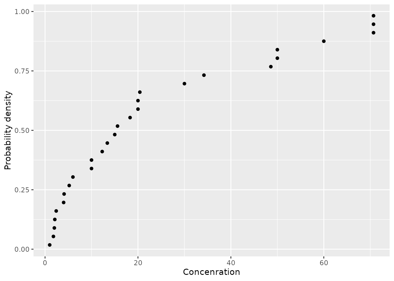

The second is geom_ssdsegments() which plots the range of censored species sensitivity data

ggplot(ccme_boron) +
  geom_ssdsegment(aes(x = Conc, xend = Conc * 2)) +
  ylab("Probability density") +
  xlab("Concenration")

The third is geom_xribbon() which plots species sensitivity confidence intervals

ggplot(boron_pred) +
  geom_xribbon(aes(xmin = lcl, xmax = ucl, y = proportion)) +
  ylab("Probability density") +
  xlab("Concenration")

And the fourth is geom_hcintersect() which plots hazard concentrations

ggplot() +
  geom_hcintersect(xintercept = c(1, 2, 3), yintercept = c(0.05, 0.1, 0.2)) +
  ylab("Probability density") +
  xlab("Concenration")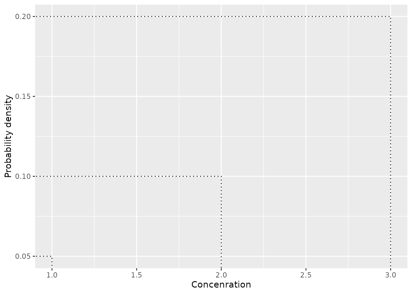

They can be combined together as follows

gp <- ggplot(boron_pred, aes(x = est)) +
  geom_xribbon(aes(xmin = lcl, xmax = ucl, y = proportion), alpha = 0.2) +
  geom_line(aes(y = proportion)) +
  geom_ssdsegment(data = ccme_boron, aes(x = Conc / 2, xend = Conc * 2)) +
  geom_ssdpoint(data = ccme_boron, aes(x = Conc / 2)) +
  geom_ssdpoint(data = ccme_boron, aes(x = Conc * 2)) +
  scale_y_continuous("Species Affected (%)", labels = scales::percent) +
  expand_limits(y = c(0, 1)) +
  xlab("Concentration (mg/L)")
print(gp + geom_hcintersect(xintercept = boron_hc5$est, yintercept = 5 / 100))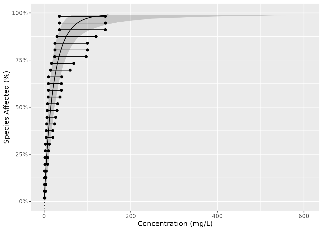

To log the x-axis add the following code.

gp <- gp + coord_trans(x = "log10") +
  scale_x_continuous(
    breaks = scales::trans_breaks("log10", function(x) 10^x),
    labels = comma_signif
  )
print(gp + geom_hcintersect(xintercept = boron_hc5$est, yintercept = 0.05))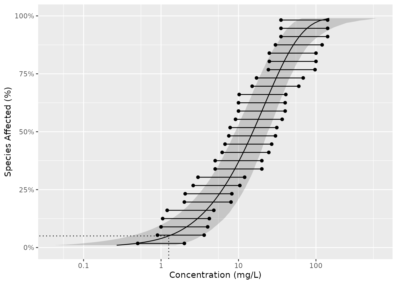

The most recent plot can be saved as a file using ggsave(), which also allows the user to set the resolution.

ggsave("file_name.png", dpi = 600)

Fitting and plotting distributions to multiple groups such taxa and/or chemicals

An elegant approach using some tidyverse packages is demonstrated below.

library(ssddata)
library(ssdtools)
library(ggplot2)
library(dplyr)
library(tidyr)
library(purrr)

boron_preds <- nest(ccme_boron, data = c(Chemical, Species, Conc, Units)) %>%
  mutate(
    Fit = map(data, ssd_fit_dists, dists = "lnorm"),
    Prediction = map(Fit, predict)
  ) %>%
  unnest(Prediction)

The resultant data and predictions can then be plotted as follows.

library(ssdtools)
library(ssddata)
ssd_plot(ccme_boron, boron_preds, xlab = "Concentration (mg/L)", ci = FALSE) +
  facet_wrap(~Group)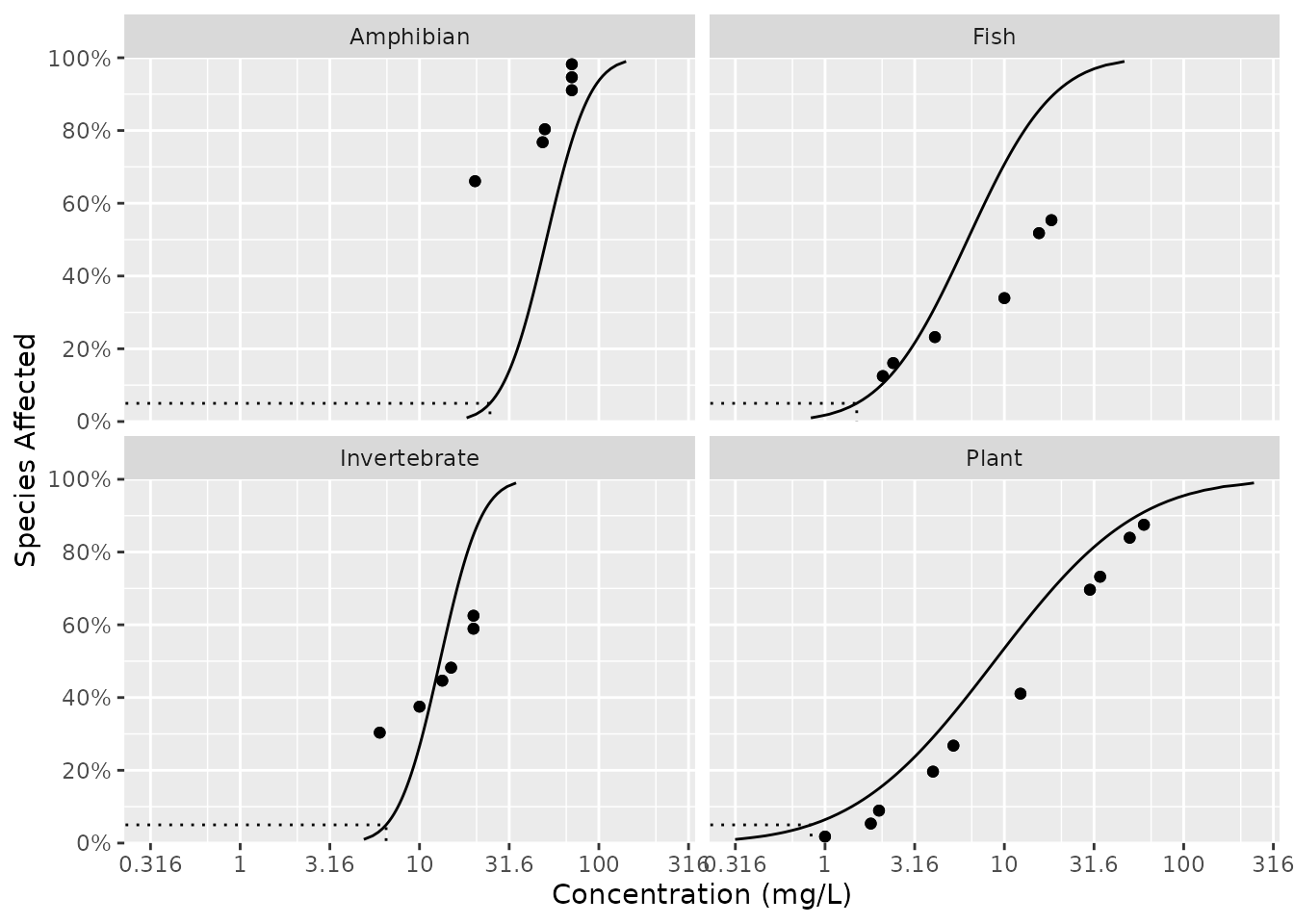

Embellishing Plots with an Exposure Distribution

For example, suppose we want to superimpose an environmental concentration cumulative distribution and compute the exposure risk as outlined in Verdonck et al. (2003).

Finding a suitable probability distribution to describe the exposure concentration is beyond the scope of this document – we will assume that this has been done elsewhere. In particular, suppose that the exposure concentration follows a log-normal distribution with a mean of -2.3 and a standard deviation of 1 on the logarithmic scale. From the exposure distribution, we construct a data frame with the concentration values and the cumulative probability of seeing this exposure or less in the environment.

Notice that some care is needed because the ssdtools plot is on the logarithmic base 10 scale and not the natural logarithm base \(e\) scale.

ex.cdf <- data.frame(Conc = exp(seq(log(.01), log(10), .1))) # generate a grid of concentrations
ex.cdf$ex.cdf <- plnorm(ex.cdf$Conc,
  meanlog = ex.mean.log,
  sdlog = ex.sd.log
) # generate the cdf

We now add this to the plot

gp +
  geom_line(data = ex.cdf, aes(x = Conc, y = ex.cdf), color = "red", linewidth = 2) +
  annotate("text",
    label = paste("Exposure distribution"),
    x = 1.08 * ex.cdf$Conc[which.max(ex.cdf$ex.cdf > 0.5)], y = 0.5, angle = 75
  )

The ssdtools package contains a function ssd_exposure() that computes the risk as defined by Verdonck et al (2003) representing the average proportion of species at risk.

set.seed(99)
ex.risk <- ssd_exposure(fits, meanlog = ex.mean.log, sdlog = ex.sd.log)
ex.risk

## [1] 0.0062416

The risk of 0.00624 can also be added to the plot in the usual way:

gp +
  geom_line(dat = ex.cdf, aes(x = Conc, y = ex.cdf), color = "red", linewidth = 2) +
  annotate("text",
    label = paste("Exposure distribution"),
    x = 1.08 * ex.cdf$Conc[which.max(ex.cdf$ex.cdf > 0.5)], y = 0.5, angle = 75
  ) +
  annotate("text",
    label = paste("Verdonck risk :", round(ex.risk, 5)),
    x = Inf, y = 0, hjust = 1.1, vjust = -.5
  )

References

Verdonck FAM, Aldenberg T, Jaworska J, Vanrolleghem PA (2003) Limitations of Current Risk Characterization Methods in Probabilistic Environmental Risk Assessment. Environmental Toxicology and Chemistry 22:2209. https://doi.org/10.1897/02-435

Licensing

The documentation is released under the CC BY 4.0 License

The code is released under the Apache License 2.0

ssdtools Team

2024-05-02