Model Averaged SSDs
ssdtools Team
2024-05-02
Source:vignettes/A_model_averaging.Rmd
A_model_averaging.RmdBackground
“Many authors have noted that there is no guiding theory in ecotoxicology to justify any particular distributional form for the SSD other than that its domain be restricted to the positive real line (Newman et al. 2000), (Zajdlik 2005), (Chapman et al. 2007), (Fox 2016). Indeed, (Chapman et al. 2007) described the identification of a suitable probability model as one of the most important and difficult choices in the use of SSDs. Compounding this lack of clarity about the functional form of the SSD is the omnipresent, and equally vexatious issue of small sample size, meaning that any plausible candidate model is unlikely to be rejected (Fox et al. 2021a). The ssdtools R package uses a model averaging procedure to avoid the need to a-priori select a candidate distribution and instead uses a measure of ‘fit’ for each model to compute weights to be applied to an initial set of candidate distributions. The method, as applied in the SSD context is described in detail in (Fox et al. 2021a), and potentially provides a level of flexibility and parsimony that is difficult to achieve with a single SSD distribution”. (Fox et al. 2021b)
Preliminaries
Before we jump into model averaging and in particular, SSD Model Averaging, let’s backup a little and consider why we average and the advantages and disadvantages of averaging.The pros and cons of averaging
We’re all familiar with the process of averaging. Indeed, averages are pervasive in everyday life - we talk of average income; mean sea level; average global temperature; average height, weight, age etc. etc. So what’s the obsession with averaging? It’s simple really - it’s what statisticians call data reduction which is just a fancy name to describe the process of summarising a lot of raw data using a small number of (hopefully) representative summary statistics such as the mean and the standard deviation. Clearly, it’s a lot easier to work with just a single mean than all the individual data values. That’s the upside. The downside is that the process of data reduction decimates your original data - you lose information in the process. Nevertheless, the benefits tend to outweigh this information loss. Indeed, much of ‘conventional’ statistical theory and practice is focused on the mean. Examples include T-tests, ANOVA, regression, and clustering. When we talk of an ‘average’ we are usually referring to the simple, arithmetic mean:\[\bar{X}=\frac{1}{n}\sum\limits_{i=1}^{n}{{{X}_{i}}}\] although we recognize there are other types of mean including the geometric mean, the harmonic mean and the weighted mean. The last of these is particularly pertinent to model averaging.
Weighted Averages
For the simple arithmetic mean, all of the individual values receive
the same weighting - they each contribute \(\frac{1}{n}\) to the summation. While this
is appropriate in many cases, it’s not useful when the components
contribute to varying degrees. An example familiar to ecotoxicologists
is that of a time-varying concentration as shown in the figure
below.

From the figure we see there are 5 concentrations going from left to
to right: \(\left\{ 0.25,0.95,0.25,0.12,0.5
\right\}\). If we were to take the simple arithmetic mean of
these concentrations we get \(\bar{X}=0.414\). But this ignores the
different durations of these 5 concentrations. Of the 170
hours, 63 were at concentration 0.25, 25 at concentration 0.95, 23 at
concentration 0.25, 23 at concentration 0.12, and 36 at concentration
0.50. So if we were to weight these concentrations by time
have:
\[{{{\bar{X}}}_{TW}}=\frac{\left(
63\cdot 0.25+25\cdot 0.95+23\cdot 0.25+23\cdot 0.12+36\cdot 0.50
\right)}{\left( 63+25+23+23+36
\right)}=\frac{56.01}{170}=0.33\]
So, our formula for a
weighted average is:\[\bar{X}=\sum\limits_{i=1}^{n}{{{w}_{i}}{{X}_{i}}}\]
with \(0\le {{w}_{i}}\le 1\) and \(\sum\limits_{i=1}^{n}{{{w}_{i}}=1}\).
Note,
the simple arithmetic mean is just a special case of the weighted mean
with \(\sum\limits_{i=1}^{n}{{{w}_{i}}=\frac{1}{n}}\)
; \(\forall i=1,\ldots ,n\)
Model Averaging
The weighted average acknowledges that the elements in the computation are not of equal ‘importance’. In the example above, this importance was based on the proportion of time that the concentration was at a particular level. Bayesians are well-versed in this concept - the elicitation of prior distributions for model parameters provides a mechanism for weighting the degree to which the analysis is informed by existing knowledge versus using a purely data-driven approach. Model averaging is usually used in the context of estimating model parameters or quantities derived from a fitted model - for example an EC50 derived from a C-R model. Let’s motivate the discussion using the following small dataset of toxicity estimates for some chemical.
#> [1] 1.73 0.57 0.33 0.28 0.30 0.29 2.15 0.80 0.76 0.54 0.42 0.83 0.21 0.18 0.59Now, suppose we have only two possibilities for fitting an SSD - both lognormal distributions. Model 1 is the LN(-1.067,0.414) distribution while Model 2 is the LN(-0.387,0.617) distribution. A plot of the empirical cdf and Models 1 and 2 is shown below.
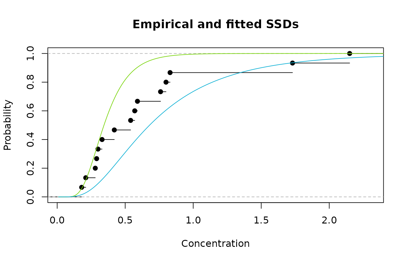
Emprirical cdf (black); Model 1(green); and Model 2 (blue)
We see that Model 1 fits well in the lower, left region and
poorly in the upper region, while the reverse is true for Model 2. So
using either Model 1 or Model 2 is going to
result in a poor fit overall. However, the obvious thing to do is to
combine both models. We could just try using 50% of
Model 1 and 50% of Model 2, but that may be sub-optimal. It turns out
that the best fit is obtained by using 44% of Model 1 and 56% of Model
2. Redrawing the plot and adding the weighted average of Models
1 and 2 is shown below.
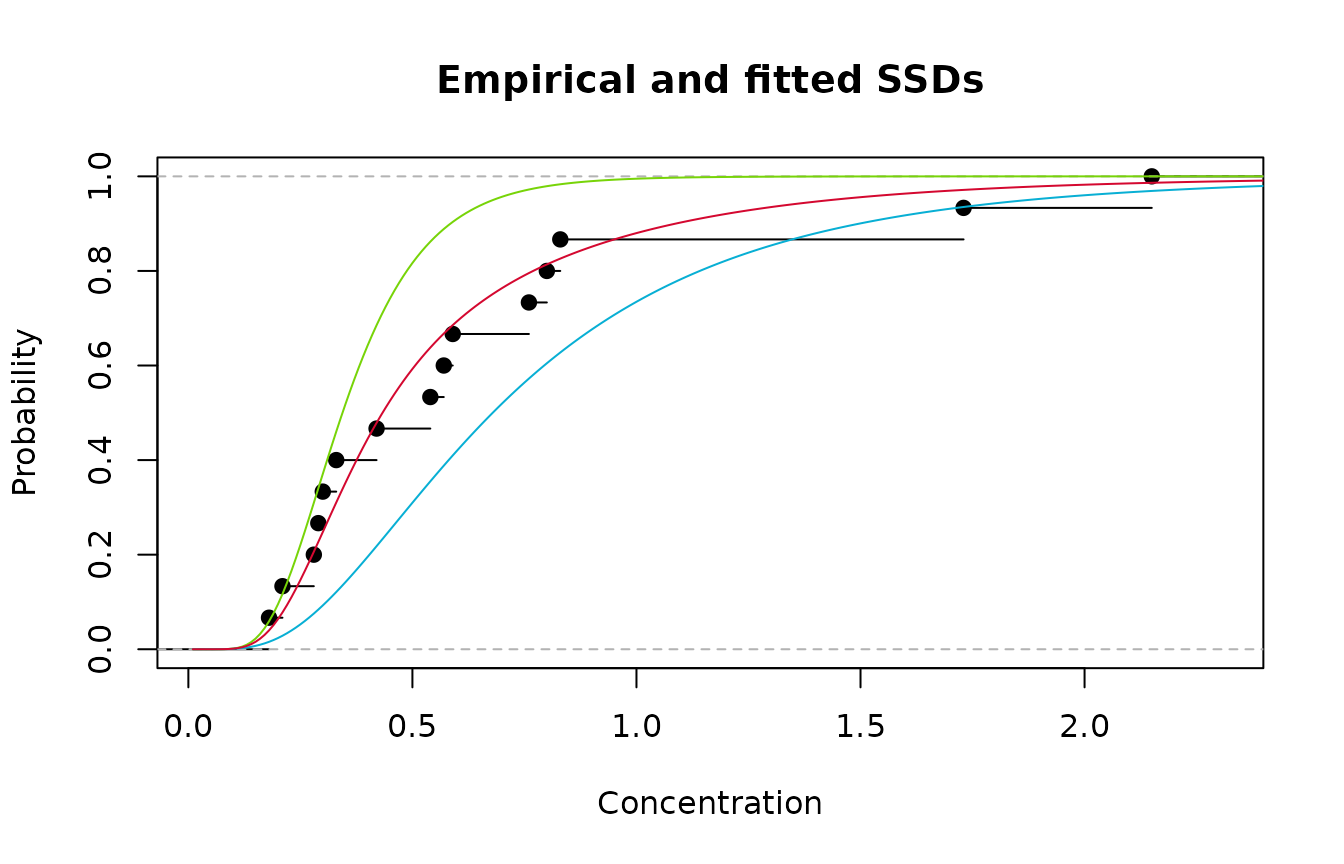
Empirical cdf (black); Model 1(green); Model 2 (blue); and averaged Model (red)
Clearly the strategy has worked - we now have an excellent
fitting SSD.What about estimation of an HC20? It’s a simple
matter to work out the individual HC20 values for
Models 1&2 using the appropriate qlnorm() function in
R. Thus we have:
# Model 1 HC20
cat("Model 1 HC20 =",qlnorm(0.2,-1.067,0.414))
#> Model 1 HC20 = 0.2428209

# Model 2 HC20
cat("Model 2 HC20 =",qlnorm(0.2,-0.387,0.617))
#> Model 2 HC20 = 0.4040243
What about the averaged distribution? An intuitively appealing
approach would be to apply the same weights to the individual
HC20 values as was applied to the respective models. That is
0.44*0.2428209 + 0.56*0.4040243 = 0.33.
So our model-averaged HC20 estimate is 0.33. As a check, we can determine the fraction affected at concentration = 0.33 - it should of course be 20%. Let’s take a look at the plot.

Something’s wrong - the fraction affected at concentration 0.33 is 30% - not the required 20%. This issue is taken up in the next section
Model Averaged SSDs
As we’ve just seen, applying the model weights to component HCx values and summing does not produce the correct result. The reason for this can be explained mathematically as follows (if your not interested in the mathematical explanation - skip ahead to the next section).The fallacy of weighting individual HCx values
The correct expression for a model-averaged SSD is: \[G\left( x \right) = \sum\limits_{i = 1}^k {{w_i}}
{F_i}\left( x \right)\] where \({F_i}\left( \cdot \right)\) is the
ith component SSD (i.e. cdf) and
wi is the weight assigned to \({F_i}\left( \cdot \right)\).
Notice
that the function \(G\left( x \right)\)
is a proper cumulative distribution function (cdf)
which means for a given quantile, x, \(G\left( x \right)\) returns the
cumulative probability: \[P\left[ {X
\leqslant x} \right]\]
Now, the incorrect approach takes a weighted sum of the
component inverse cdf’s, that is:
Now, the correct method of determining the HCx is to work with the proper model-averaged cdf \(G\left( x \right)\). This means finding the inverse function \({G^{ - 1}}\left( p \right)\). We’ll address how we do this in a moment.
The reason why \(H\left( p \right)\) does not return the correct result is because of the implicit assumption that the inverse of \(G\left( x \right)\) is equivalent to \(H\left( p \right)\). This is akin to stating the inverse of a sum is equal to the sum of the inverses i.e. \[\sum\limits_{i = 1}^n {\frac{1}{{{X_i}}}} = \frac{1}{{\sum\limits_{i = 1}^n {{X_i}} }}{\text{ ???}}\]For the mathematical nerds: There are some very special cases where the above identity does in fact hold, but for that you need to use complex numbers.
For example, consider two complex numbers \[{\text{a = }}\frac{{\left( {5 - i} \right)}}{2}{\text{ and }}b = - 1.683 - 1.915i\] It can be shown that \[\frac{1}{{a + b}} = \frac{1}{a} + \frac{1}{b} = 0.126 + 0.372i\]
Back to the issue at hand, and since we’re not dealing with complex numbers, it’s safe to say:\[{G^{ - 1}}\left( p \right) \ne H\left( p \right)\]
If you need a visual demonstration, we can plot \(G\left( x \right)\) and the inverse of \(H\left( p \right)\) both as functions of x (a quantile) for our two-component lognormal distribution above.
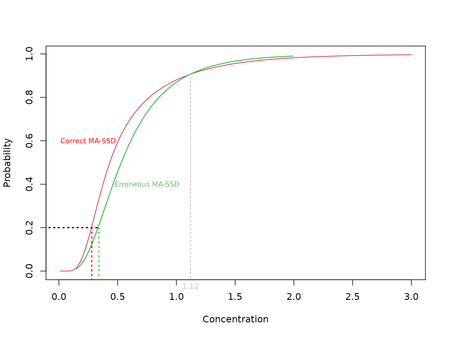
WE next discuss the use of a model-averaged SSD to obtain the correct model-averaged HCx.
Computing a model-averaged HCx
A proper HCx needs to satisfy what David Fox refers to as the inversion principle.More formally, the inversion principle states that an HCx (denoted as \({\varphi _x}\)) must satisfy the following:
\[df\left( {{\varphi _x}} \right) = x\quad \quad and\quad \quad qf\left( x \right) = {\varphi _x}\]
where \(df\left( \cdot \right)\) is a model-averaged distribution function (i.e. SSD) and \(qf\left( \cdot \right)\) is a model-averaged quantile function. For this equality to hold, it is necessary that \(qf\left( p \right) = d{f^{ - 1}}\left( p \right)\).
So, in our example above, the green curve was taken to be \(qf\left( x \right)\) and this was used to derive \({\varphi _x}\) but the fraction affected \(\left\{ { = df\left( {{\varphi _x}} \right)} \right\}\) at \({\varphi _x}\) is computed using the red curve.
In ssdtools the following is a check that the inversion
principle holds:
# Obtain a model-averaged HCx using the ssd_hc() function
hcp<-ssd_hc(x, p = p)
# Check that the inversion principle holds
ssd_hp(x, hcp, multi_est = TRUE) == p   # this should result in logical `TRUE`
Note: if the multi_est argument is set to
FALSE the test will fail.
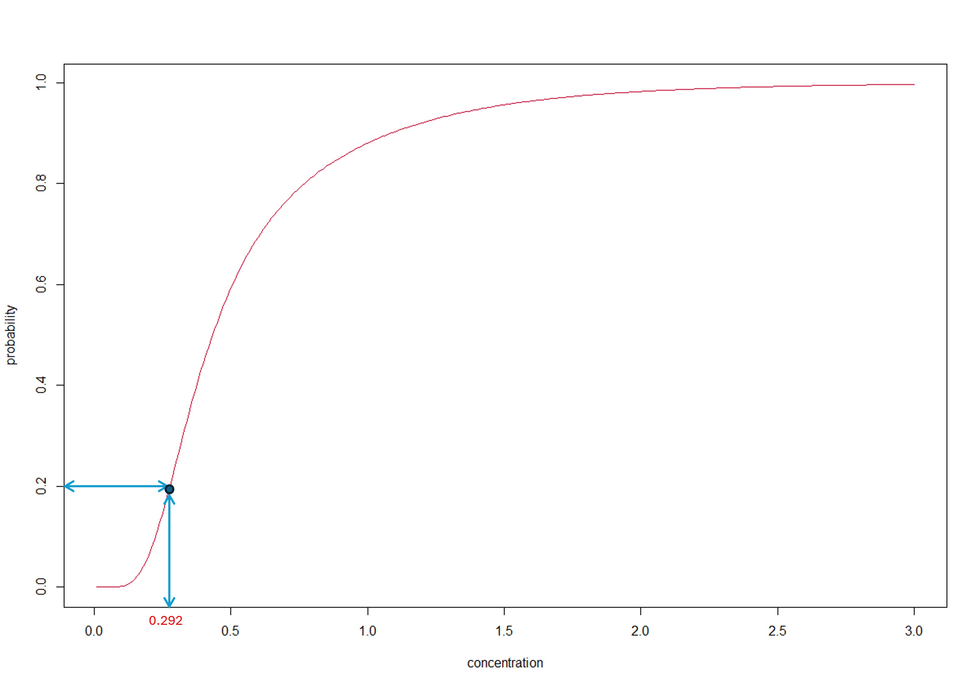
The inversion principle ensures that we only use a single distribution function to compute both the HCx and the fraction affected. Referring to the figure below, the HCx is obtained from the MA-SSD (red curve) by following the → arrows while the fraction affected is obtained by following the ← arrows.
Finally, we’ll briefly discuss how the HCx is computed in
R using the same method as has been implemented in
ssdtools.
Computing the HCx in
R/ssdtools
Recall, our MA-SSD was given as \[G\left( x
\right) = \sum\limits_{i = 1}^k {{w_i}} {F_i}\left( x \right)\]
and an HCx is obtained from the MA-SSD by essentially working
‘in reverse’ by starting at a value of \(x\) on the vertical scale
in the Figure above and following the → arrows and reading off the
corresponding value on the horizontal scale.
Obviously, we need to be able to ‘codify’ this process in R
(or any other computer language).
Mathematically this is equivalent
to seeking a solution to the following equation:\[{x:G\left( x \right) = p}\] or,
equivalently:\[x:G\left( x \right) - p =
0\] for some fraction affected, \(p\).
Finding the solution to this last equation is referred to as finding the root(s) of the function \(G\left( x \right)\) or, as is made clear in the figure below, finding the zero-crossing of the function \(G\left( x \right)\) for the case \(p=0.2\).

In R finding the roots of \(x:G\left( x \right) - p = 0\) is achieved
using the uniroot() function.
Help on the uniroot function can be found here
Where do the model-averaged weights come from?
This is a little more complex, although we’ll try to provide a non-mathematical explanation. For those interested in going deeper, a more comprehensive treatment can be found in (Burnham and Anderson 2002) and (Fletcher 2018) as well as this on-line course .
This time, we’ll look at fitting a gamma, lognormal, and pareto distribution to our sample data:
#> [1] 1.73 0.57 0.33 0.28 0.30 0.29 2.15 0.80 0.76 0.54 0.42 0.83 0.21 0.18 0.59
The adequacy (or otherwise) of a fitted model can be assessed
using a variety of numerical measures known as
goodness-of-fit or GoF statistics. These are invariably
based on a measure of discrepancy between the emprical data and the
hypothesized model. Common GoF statistics used to test whether the
hypothesis of some specified theoretical probability distribution is
plausible for a given data set include: Kolmogorov-Smirnov test;
Anderson-Darling test; Shapiro-Wilk test;and Cramer-von Mises test.
The
Cramer-von Mises test is a good choice and is readily performed
using the cvm.test() function in the goftest
package in R as follows:
dat<-data.frame(Conc=c(1.73,0.57,0.33,0.28,0.3,0.29,2.15,0.8,0.76,0.54,0.42,0.83,0.21,0.18,0.59))
library(goftest)
library(EnvStats)  # this is required for the Pareto cdf (ppareto)

# Examine the fit for the gamma distribution (NB: parameters estimated from the data)
cvm.test(dat$Conc,null = "pgamma",shape = 2.0591977,scale = 0.3231032,estimated = TRUE)

# Examine the fit for the lognormal distribution (NB: parameters estimated from the data)
cvm.test(dat$Conc,null = "plnorm",meanlog=-0.6695120,sd=0.7199573,estimated = TRUE)

# Examine the fit for the Pareto distribution (NB: parameters estimated from the data)
cvm.test(dat$Conc,null = "ppareto",location = 0.1800000,shape    = 0.9566756,estimated = TRUE)
Cramer-von Mises test of goodness-of-fit
Braun's adjustment using 4 groups
Null hypothesis: Gamma distribution
with parameters shape = 2.0591977, scale = 0.3231032
Parameters assumed to have been estimated from data
data: dat$Conc
omega2max = 0.34389, p-value = 0.3404
Cramer-von Mises test of goodness-of-fit
Braun's adjustment using 4 groups
Null hypothesis: log-normal distribution
with parameter meanlog = -0.669512
Parameters assumed to have been estimated from data
data: dat$Conc
omega2max = 0.32845, p-value = 0.3719
Cramer-von Mises test of goodness-of-fit
Braun's adjustment using 4 groups
Null hypothesis: distribution ‘ppareto’
with parameters location = 0.18, shape = 0.9566756
Parameters assumed to have been estimated from data
data: dat$Conc
omega2max = 0.31391, p-value = 0.4015From this output and using a level of significance of \(p = 0.05\), we see that none of the
distributions is implausible. However, if forced to choose just
one distribution, we would choose the Pareto distribution
(smaller values of the omega2max statistic are better).
However, this does not mean that the gamma and lognormal distributions
are of no value in describing the data. We can see from the plot below,
that in fact both the gamma and lognormal distributions do a reasonable
job over the range of toxicity values. The use of the Pareto may be a
questionable choice given it is truncated at 0.18 (which is the minimum
value of our toxicity data).
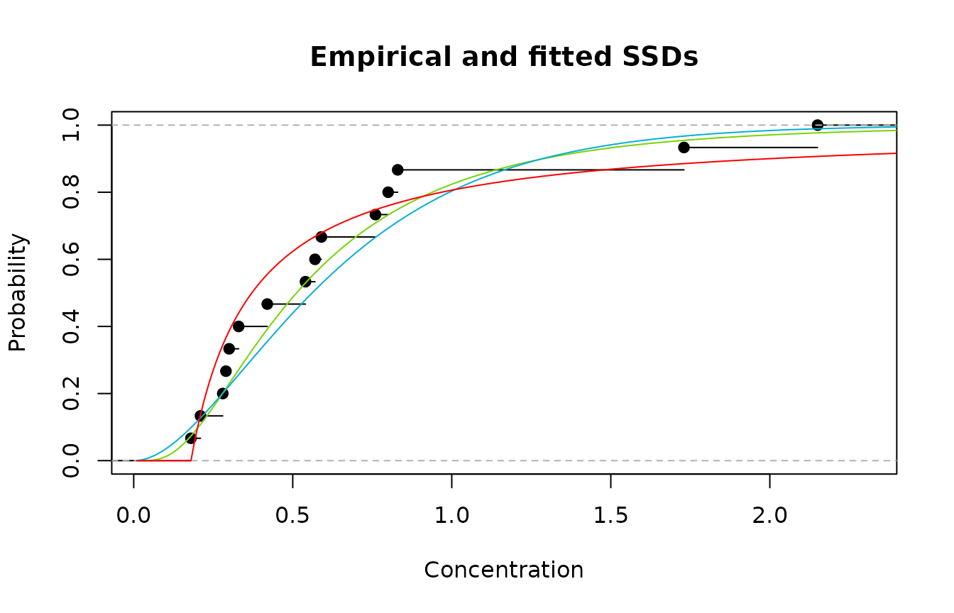
Emprirical cdf (black); lognormal (green); gamma (blue); and Pareeto (red)
As in the earlier example, we might expect to find a better fitting
distribution by combining all three distributions using a
weighted SSD. The issue we face now is how do we choose the
weights to reflect the relative fits of the three distributions?
Like all tests of statistical significance, a p-value is
computed from the value of the relevant test statistic - in
this case, the value of the omega2max test statistic. For
this particular test, it’s a case of the smaller the better. From
the output above we see that the omega2max values are \(0.344\) for the gamma distribution, \(0.328\) for the lognormal distribution, and
\(0.0.314\) for the Pareto
distribution.
We might somewhat naively compute the relative weights as:
\({w_1} = \frac{{{{0.344}^{ - 1}}}}{{\left(
{{{0.344}^{ - 1}} + {{0.328}^{ - 1}} + {{0.314}^{ - 1}}} \right)}} =
0.318\) \({w_2} =
\frac{{{{0.328}^{ - 1}}}}{{\left( {{{0.344}^{ - 1}} + {{0.328}^{ - 1}} +
{{0.314}^{ - 1}}} \right)}} = 0.333\) and \({w_3} = \frac{{{{0.314}^{ - 1}}}}{{\left(
{{{0.344}^{ - 1}} + {{0.328}^{ - 1}} + {{0.314}^{ - 1}}} \right)}} =
0.349\)
(we use reciprocals since smaller values
of omega2max represent better fits). As will be seen
shortly - these are incorrect.
However, being based on a simplistic measure of discrepancy between the
observed and hypothesized distributions, the
omega2max statistic is a fairly ‘blunt instrument’ and has
no grounding in information theory which is the basis for
determining the weights that we seek.
A discussion of information theoretic methods for
assessing goodness-of-fit is beyond the scope of this vignette.
Interested readers should consult (Burnham and
Anderson 2002) or the on-line
course. A commonly used metric to determine the model-average
weights is the Akaike Information Criterion or AIC.
The formula for the \(AIC\) is: \[AIC = 2k - 2\ln \left( \ell \right)\]
The likelihood for our three distributions can be computed in
R as follows:
sum(log(EnvStats::dpareto(dat$Conc,location = 0.1800000, shape=0.9566756)))
#> [1] -5.621683
sum(log(dgamma(dat$Conc,shape = 2.0591977,scale = 0.3231032)))
#> [1] -7.020597
sum(log(dlnorm(dat$Conc, meanlog = -0.6695120,sdlog   =  0.7199573)))
#> [1] -5.812947
From which the AIC values readily follow:
#> AIC for gamma distribution = 18.04119
#> AIC for lognormal distribution = 15.62589
#> AIC for Pareto distribution = 15.24337
As with the omega2max statistic,
smaller values of AIC are better. Thus, a
comparison of the AIC values above gives the ranking of distributional
fits (best to worst) as: Pareto > lognormal > gamma
Computing model weights from the AIC
We will simply provide a formula for computing the model weights from
the AIC values. More detailed information can be found here.
The AIC for the ith distribution fitted to the data is \[AI{C_i} = 2{k_i} - 2\ln \left( {{L_i}} \right) \] where \({L_i}\) is the ith likelihood and \({k_i}\) is the number of parameters for the ith distribution. Next, we form the differences:\[{\Delta _i} = AI{C_i} - AI{C_0}\] where \(AI{C_0}\) is the AIC for the best-fitting model (i.e.\(AI{C_0} = \mathop {\min }\limits_i \left\{ {AI{C_i}} \right\}\) ). The model-averaged weights \({w_i}\) are then computed as:
The model-averaged weights for the gamma, lognormal, and Pareto
distributions used in the previous example can be computed ‘manually’ in
R as follows:
dat<-c(1.73,0.57,0.33,0.28,0.3,0.29,2.15,0.8,0.76,0.54,0.42,0.83,0.21,0.18,0.59)
aic<-NULL
k<-2  # number of parameters for each of the distributions


aic[1]<-2*k-2*sum(log(dgamma(dat,shape = 2.0591977,scale = 0.3231032))) # Gamma distribution

aic[2]<-2*k-2*sum(log(dlnorm(dat, meanlog = -0.6695120,sdlog   =  0.7199573)))  # lognormal distribution

aic[3]<-2*k-2*sum(log(EnvStats::dpareto(dat,location = 0.1800000, shape=0.9566756))) # Pareto distribution

delta<-aic-min(aic)  #  compute the delta values

aic.w<-exp(-0.5*delta); aic.w<-round(aic.w/sum(aic.w),4)

cat(" AIC weight for gamma distribution =",aic.w[1],"\n",
    "AIC weight for lognormal distribution =",aic.w[2],"\n",
    "AIC weight for pareto distribution =",aic.w[3],"\n")
AIC weight for gamma distribution = 0.1191
AIC weight for lognormal distribution = 0.3985
AIC weight for pareto distribution = 0.4824 Finally, let’s look at the fitted model-averaged SSD:
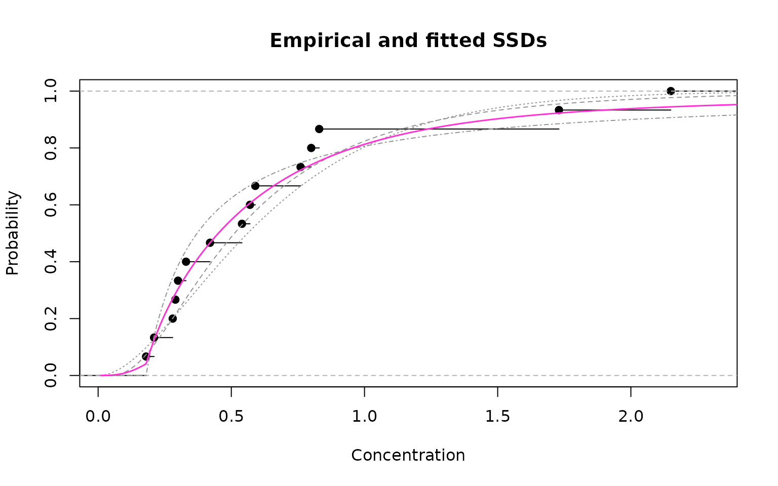
Empirical cdf (black) and model-averaged fit (magenta)
As can be seen from the figure above, the model-averaged fit provides a very good fit to the empirical data.
Correcting for distributions having differing numbers of parameters
In deriving the AIC, Akaike had to make certain, strong assumptions. In addition, the bias factor (the \(2k\) term) was derived from theoretical considerations (such as mathematical expectation) that relate to infinite sample sizes. For small sample sizes, the AIC is likely to select models having too many parameters (i.e models which over-fit) In 1978, Sugiura proposed a modification to the AIC to address this problem, although it too relied on a number of assumptions. This ‘correction’ to the AIC for small samples (referred to as \(AI{{C}_{c}}\)) is:
\[AI{{C}_{c}}=AIC+\frac{2{{k}^{2}}+2k}{n-k-1}\]where n is the sample size and k is the number of parameters.
It is clear from the formula for \(AI{{C}_{c}}\) that for \(n\gg k\), \(AI{{C}_{c}}\simeq AIC\). The issue of
sample size is ubiquitous in statistics, but even more so in
ecotoxicology where logistical and practical limitations invariably mean
we are dealing with (pathologically) small sample sizes. There are no
hard and fast rules as to what constitutes an appropriate
sample size for SSD modelling. However, Professor David Fox’s personal
rule of thumb which works quite well is:
Since most of the common SSD models are 2-parameter, we should be
aiming to have a sample size of at least 11. For 3-parameter models
(like the Burr III), the minimum sample size is 16 and if we wanted to
fit a mixture of two, 2-parameter models (eg.
logNormal-logNormal or logLogistic-logLogistic) the
sample size should be at least 26. Sadly, this is rarely the
case in practice!
Model-Averaging in ssdtools
Please see the Getting
started with ssdtools vignette for examples of obtaining
model-averaged HCx values and predictions using
ssdtools.
References
Licensing
Copyright 2024 Province of British Columbia, Environment and Climate Change Canada, and Australian Government Department of Climate Change, Energy, the Environment and Water
The documentation is released under the CC BY 4.0 License
The code is released under the Apache License 2.0