Species Sensitivity Distributions • ssdtools

ssdtools is an R package to fit and plot Species Sensitivity Distributions (SSD).

SSDs are cumulative probability distributions which are fitted to toxicity concentrations for different species as described by Posthuma et al. (2001). The ssdtools package uses Maximum Likelihood to fit distributions such as the log-normal, log-logistic, log-Gumbel (also known as the inverse Weibull), gamma, Weibull and log-normal log-normal mixture. Multiple distributions can be averaged using Akaike Information Criteria. Confidence intervals on hazard concentrations and proportions are produced by bootstrapping.

Installation

To install the latest version from CRAN

install.packages("ssdtools")

To install the latest development version from GitHub

# install.packages("remotes")
remotes::install_github("bcgov/ssdtools")

Introduction

The dependency ssddata provides a example data sets for several chemicals including Boron.

library(ssdtools)
ssddata::ccme_boron
#> # A tibble: 28 × 5
#>    Chemical Species                  Conc Group        Units
#>    <chr>    <chr>                   <dbl> <fct>        <chr>
#>  1 Boron    Oncorhynchus mykiss       2.1 Fish         mg/L 
#>  2 Boron    Ictalurus punctatus       2.4 Fish         mg/L 
#>  3 Boron    Micropterus salmoides     4.1 Fish         mg/L 
#>  4 Boron    Brachydanio rerio        10   Fish         mg/L 
#>  5 Boron    Carassius auratus        15.6 Fish         mg/L 
#>  6 Boron    Pimephales promelas      18.3 Fish         mg/L 
#>  7 Boron    Daphnia magna             6   Invertebrate mg/L 
#>  8 Boron    Opercularia bimarginata  10   Invertebrate mg/L 
#>  9 Boron    Ceriodaphnia dubia       13.4 Invertebrate mg/L 
#> 10 Boron    Entosiphon sulcatum      15   Invertebrate mg/L 
#> # ℹ 18 more rows

The six default distributions are fit using ssd_fit_dists()

fits <- ssd_fit_dists(ssddata::ccme_boron)

and can be quickly plotted using autoplot

autoplot(fits)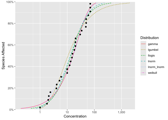

The goodness of fit can be assessed using ssd_gof

ssd_gof(fits)
#> # A tibble: 6 × 9
#>   dist           ad     ks    cvm   aic  aicc   bic delta weight
#>   <chr>       <dbl>  <dbl>  <dbl> <dbl> <dbl> <dbl> <dbl>  <dbl>
#> 1 gamma       0.440 0.117  0.0554  238.  238.  240. 0.005  0.357
#> 2 lgumbel     0.829 0.158  0.134   244.  245.  247. 6.56   0.013
#> 3 llogis      0.487 0.0994 0.0595  241.  241.  244. 3.39   0.066
#> 4 lnorm       0.507 0.107  0.0703  239.  240.  242. 1.40   0.177
#> 5 lnorm_lnorm 0.320 0.116  0.0414  240.  243.  247. 4.98   0.03 
#> 6 weibull     0.434 0.117  0.0542  238.  238.  240. 0      0.357

and the model-averaged 5% hazard concentration estimated by bootstrapping using ssd_hc.

set.seed(99)
hc5 <- ssd_hc(fits, ci = TRUE)
print(hc5)
#> # A tibble: 1 × 11
#>   dist    proportion   est    se   lcl   ucl    wt method    nboot pboot samples
#>   <chr>        <dbl> <dbl> <dbl> <dbl> <dbl> <dbl> <chr>     <dbl> <dbl> <I<lis>
#> 1 average       0.05  1.26 0.781 0.407  3.29     1 parametr…  1000 0.999 <dbl>

To bootstrap in parallel set future::plan(). For example:

future::multisession(workers = 2)
hc5 <- ssd_hc(fits, ci = TRUE)

Model-averaged predictions complete with confidence intervals can also be estimated by parametric bootstrapping using the stats generic predict. To perform bootstrapping for each distribution in parallel register the future backend and then select the evaluation strategy.

doFuture::registerDoFuture()
future::plan(future::multisession)

set.seed(99)
boron_pred <- predict(fits, ci = TRUE)

The predictions can be plotted together with the original data using ssd_plot.

library(ggplot2)

theme_set(theme_bw())

ssd_plot(ssddata::ccme_boron, boron_pred,
  shape = "Group", color = "Group", label = "Species",
  xlab = "Concentration (mg/L)", ribbon = TRUE
) +
  expand_limits(x = 3000) +
  scale_colour_ssd()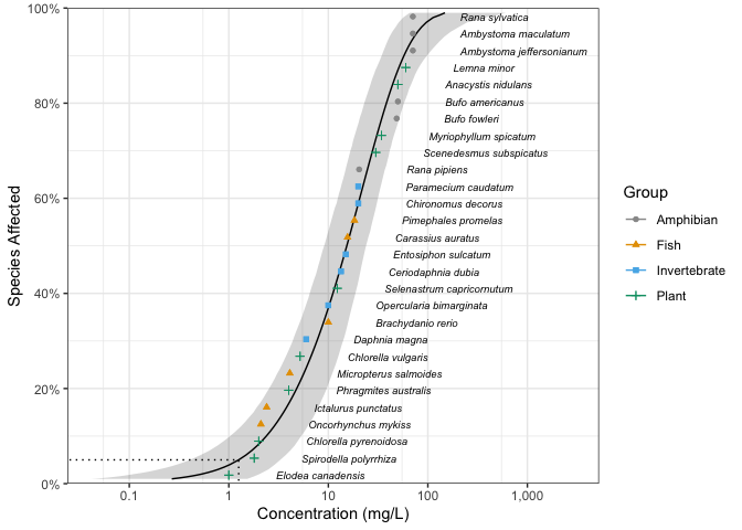

References

Posthuma, L., Suter II, G.W., and Traas, T.P. 2001. Species Sensitivity Distributions in Ecotoxicology. CRC Press.

Information

Get started with ssdtools at https://bcgov.github.io/ssdtools/articles/ssdtools.html.

A shiny app to allow non-R users to interface with ssdtools is available at https://github.com/bcgov/shinyssdtools.

For the latest changes visit NEWS.

The citation for the shiny app:

Dalgarno, S. 2021. shinyssdtools: A web application for fitting Species Sensitivity Distributions (SSDs). JOSS 6(57): 2848. https://joss.theoj.org/papers/10.21105/joss.02848.

The ssdtools package was developed as a result of earlier drafts of:

Schwarz, C., and Tillmanns, A. 2019. Improving Statistical Methods for Modeling Species Sensitivity Distributions. Province of British Columbia, Victoria, BC.

For recent developments in SSD modeling including a review of existing software see:

Fox, D.R., et al. 2021. Recent Developments in Species Sensitivity Distribution Modeling. Environ Toxicol Chem 40(2): 293–308. https://doi.org/10.1002/etc.4925.

The CCME data.csv data file is derived from a factsheet prepared by the Canadian Council of Ministers of the Environment. See the data-raw folder for more information.

Getting Help or Reporting an Issue

To report bugs/issues/feature requests, please file an issue.

How to Contribute

If you would like to contribute to the package, please see our CONTRIBUTING guidelines.

Code of Conduct

Please note that the ssdtools project is released with a Contributor Code of Conduct. By contributing to this project, you agree to abide by its terms.

Licensing

The documentation is released under the CC BY 4.0 License

The code is released under the Apache License 2.0