The climr mosaic of North American climatologies
methods_mosaic.Rmd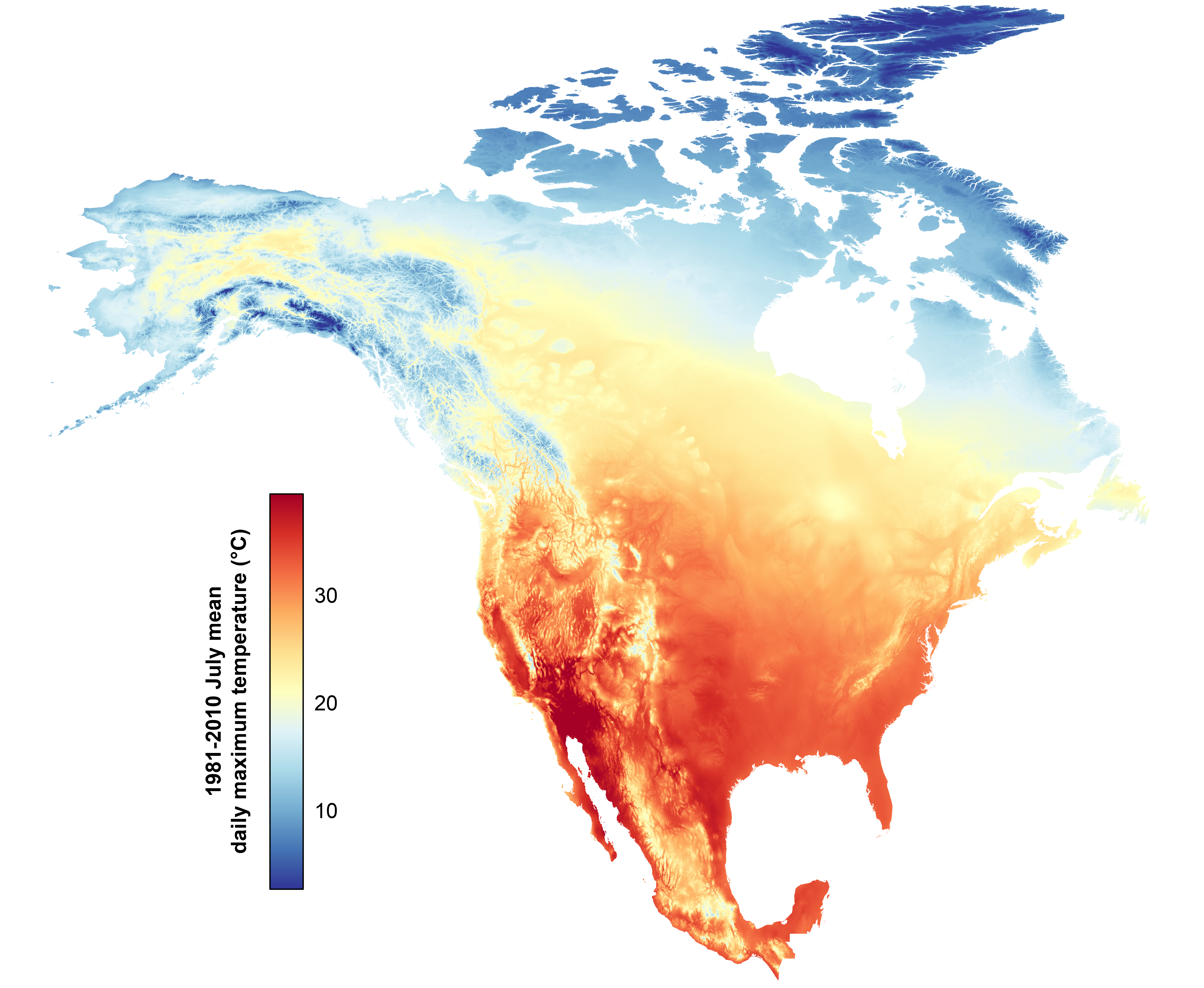
Introduction
High-quality gridded climatologies (climate maps) of North America are not currently available, despite the availability of high-quality climate maps for BC and the continental US (the PRISM maps; Daly et al. (2008)). Existing seamless maps made with a consistent methodology across North America (WorldClim, Daymet, and CHELSA) exhibit unacceptable artefacts in the complex topography of the western Cordillera. Analysts conducting cross-border studies are faced with the dilemma of introducing boundary artefacts associated with combining high-quality and low-quality products from different jurisdictions, or alternatively foregoing high-quality climate data to achieve cross-border continuity by using a lower-quality product.
The need for a relatively seamless mosaic of the best available
gridded climatologies motivated the development of the ClimateNA mosaic
of 1961-1990 normals for North America (Wang et
al. (2016)), which has been widely
used for over a decade as part of the ClimateNA downscaling product. During
the development of climr, we identified several
opportunities to complement the ClimateNA mosaic with an alternative
mosaic:
Incorporate the recently developed 800m-resolution PRISM maps for Alaska (Daly et al. 2018);
Use predictive models to blend outside the boundaries of PRISM products, to avoid degrading these high-quality products by blending with lower-quality products inside the PRISM domains;
Compile source climatologies exclusively of the 1981-2010 period, to avoid artefacts associated with adjusting for different normal periods in the source data;
Use a single product (Daymet) for central and eastern North America to provide users with a seamless map for cross-border analyses in that region; and
Compile a mosaic at higher resolution (2.5km instead of ClimateNA’s 4km map) to conserve complex elevational relationships (e.g. valley inversions) and precipitation patterns.
In this article, we describe the method for development of the climr
mosaic of 1981-2010 North American Climatologies. We highlight some
regions where this new mosaic provides substantial improvement over the
ClimateNA mosaic. However, there are many regions where the ClimateNA
mosaic provides complementary information. For example, ClimateNA
provides a mosaic of the US PRISM and Worldclim maps for eastern North
America, which users may deem preferable to climr’s Daymet climatology
for some purposes. Also, since the ClimateNA maps are stored at lower
resolution (4km instead of climr’s 2.5km), their download speed and
cache size is 2.5 times less than the climr mosaic. For these reasons,
climr::downscale() provides the option to downscale using
either the climr mosaic or the ClimateNA mosaic
(which_refmap = c("refmap_climr", "refmap_climatena")).
Methods
The climr mosaic is a composite of the 1981-2010 gridded climate maps from the following sources (Figure 1):
PRISM for Western US—The Parameter-elevation Regressions on Independent Slopes Model (PRISM; Daly et al. (2008)) maps are recognized as the highest-quality gridded climatological normals for the contiguous United States. We blended the US PRISM with BC PRISM emulator (explained below) between latitudes 48oN and 49oN.
British Columbia PRISM—The BC PRISM (Pacific Climate Impacts Consortium (2014)) is developed by the Pacific Climate Impacts Consortium in collaboration with the PRISM Climate Group (Oregon State University). It generally is highly compatible with the US and Alaska PRISM products, with exceptions noted in the Discussion section. The blending with the PRISM emulator along the northern, eastern, and southern BC boundary does not compromise the integrity of the BC PRISM since the emulator replicates the PRISM map in the blending region.
Alaska PRISM—The PRISM 1981-2010 climatological maps for Alaska (Daly et al. 2018) are the best available product, as a result of exhaustive station data compilation and local expert review, and are compatible with the BC PRISM.
Daymet for eastern North America and Mexico—While the US PRISM is likely preferable to Daymet over the continental US, Daymet (Thornton et al. (2021)) provides north-south continuity across Canada, USA, and Mexico. Daymet was chosen over other North American gridded climatologies (WorldClim and CHELSA) due to its relative quality and the availability of a 1981-2010 normal period.
PRISM Emulator in Yukon and Northwest Territories—We evaluated all available climatological maps for the Yukon and Northwest Territories (WorldClim, CHELSA, Daymet, NRCAN ANUSPLIN, and Western Canadian 4km 1961-1990 PRISM). None of these products were of acceptable quality due to very low weather station density. To provide a PRISM-compatible estimation of climate in this region, we trained deep learning models on the BC and Alaska PRISM maps and predicted them into the Yukon and NWT. This method is described in more detail below.
Predictive blending in Northern Mexico—The US PRISM and Daymet maps require blending at the US-Mexico border to avoid boundary artefacts. Rather than blending Daymet into the US PRISM, which would degrade the PRISM map, we used machine learning (Random Forest regression) to interpolate between PRISM and Daymet in a broad swath of Northern Mexico. This is a less sophisticated approach to PRISM emulation than used in the Yukon and NWT, but it is much more computationally efficient and produced acceptable results. This method is described in more detail below.
20km Coastal buffer—We extended the coastal climate values outwards into the ocean to a distance of 20km from shore. We retained existing coastal buffers present in the PRISM products and extended their outer limit where necessary. This buffer ensures climate values are available in outer coastal land areas, but is not intended to estimate temperature and precipitation over the ocean.
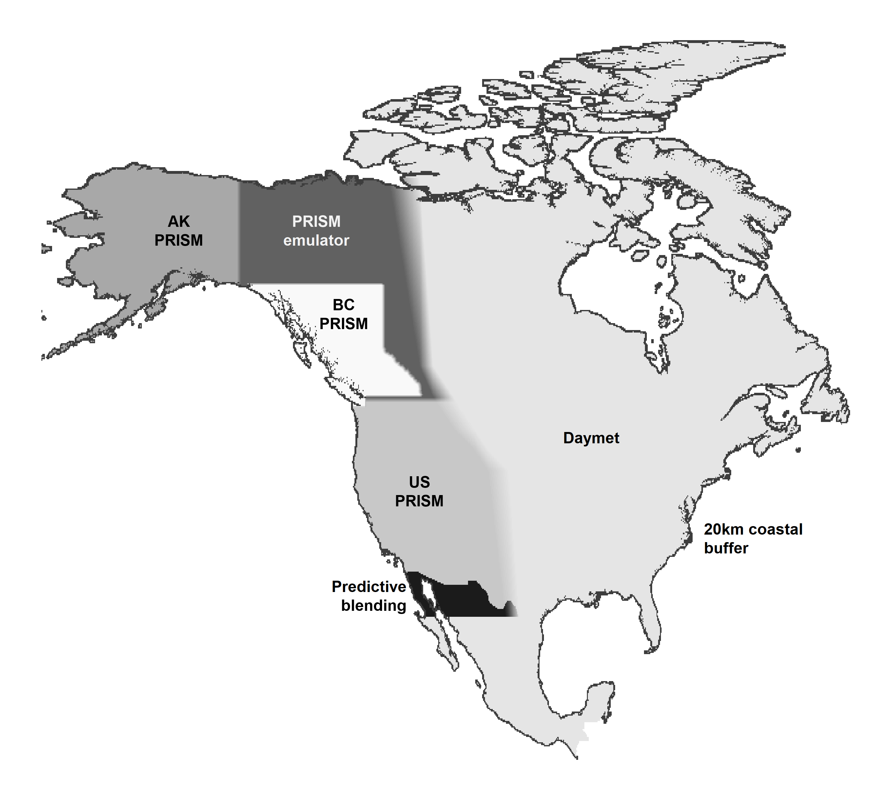
Figure 1. Elements of the climr mosaic of 1981-2010 climatologies. PRISM and Daymet are publicly available datasets. The PRISM Emulator and predictive blending were developed as part of the climr mosaic method and are described in this article. Blending between products is as shown.
PRISM emulator for the Yukon and Northwest Territories
Generative Adversarial Networks (GANs; Goodfellow et al. (2014)) are a deep learning technique originally developed for computer vision that has recently been applied to downscaling hourly weather simulations. While this approach has not been applied to climate mapping, it is appealing for this application because of its ability to make predictions of spatial patterns, rather than just point estimates. In this way, GANs can be used to emulate the spatial structures of a climatological mapping technique such as PRISM and thus provide a more seamless extrapolation of PRISM mapping into unmapped regions. While GAN-predicted climatologies are not a substitute for supervised climatological maps such as PRISM, they provide an interim solution where acceptable climate maps have not been developed, as in the Yukon and Northwest Territories.
We used a stochastic implementation of GANs (Daust and Monahan (2024)) to interpolate between the Alaska/BC PRISM maps and the Daymet maps east of longitude 112oE. One GAN model was created for each climate variable (e.g., January precipitation). The PRISM and Daymet maps for the target variable were combined into a predictand layer. As predictors, we used the WorldClim (Fick and Hijmans (2017)) climatology for the target variable as well as latitude, longitude, elevation, and coastal proximity. We ran each GAN to 150 epochs (training iterations), as trials indicated that further epochs were generally not warranted. We created three stochastic models for the months of March, June, September, and December as a means of mapping prediction uncertainty. Our models of precipitation exhibited artefacts along the arctic coast that required local substitution with a random forest prediction.
Evaluation and refinement of the PRISM emulator method is ongoing. It would likely be preferable to use weather model simulations (such as ERA5 and/or the Weather Research and Forecasting (WRF) model) as predictor variables rather than WorldClim, which likely confounds training due to spatially inconsistent climate mapping. Further, we intend to produce multiple realizations of all months (not just four) to provide comprehensive uncertainty mapping. Finally, we need to resolve the artefacts in predicted precipitation along the arctic coast.
Predictive blending for northern Mexico
The objective of predictive blending was to produce a seamless transition from the US PRISM to Daymet south of the US Border, to avoid compromising the integrity of the US PRISM. We trained one Random Forest (Breiman (2001)) regression model for each variable. The US PRISM south of 35oN and Daymet between 25-28oN were combined into a predictand layer. As predictors for each variable, we used the Daymet and WorldClim (Fick and Hijmans (2017)) climatologies for Tmin, Tmax, and precipitation of the target month and the two adjacent months (i.e., Jan-Feb-Mar for the target month of February); using multivariate climate predictors allowed the exclusion of latitude and longitude as predictors, which caused prediction artefacts during trials. Daymet contains precipitation artefacts on the Baja peninsula; for this small region we trained a separate model to blend PRISM precipitation into WorldClim precipitation.
Grid resolution
We aggregated the BC PRISM 30-arcsecond (approx 800m) grid to
90-arcsecond (approx. 2.5km) resolution and extended this grid to North
America. All other products were resampled to this grid using bilinear
interpolation. The 2.5km grid scale reduces downloading and storage by a
factor of 9, while retaining sufficient information for the original
PRISM and Daymet temperature maps to be recreated at 800m and finer
resolutions through climr’s elevation adjustment with inferred lapse
rates. climr does not apply an elevation adjustment to
precipitation, and as a result the spatial pattern of PRISM
precipitation is slightly degraded at this coarser resolution (see Figure 4. We are assessing whether the finer-resolution
details of PRISM precipitation are warranted.
Results
This section provides a brief illustration of the climr mosaic in
case study regions. ClimateNA output, sourced from a direct query to
ClimateNA (Wang et al. (2016)), is provided for comparison since
the ClimateNA mosaic is available in climr as an
alternative reference climatology.
Yukon Territory
Figure 2 (left panel) illustrates the challenge of combining climate maps made using different methodologies (i.e., PRISM vs Daymet) in a region of very low station density. While Daymet and PRISM have similar January temperatures (Tmax) at low elevations where weather stations are located, they have opposite lapse rates resulting in divergent temperatures at higher elevations (Daymet colder and PRISM warmer). In addition, the automated lapse rate calculation in Daymet produces regions of no elevational variation in temperature. In short, Daymet and PRISM are incompatible; blending them would degrade PRISM in the blending zones and create a discontinuity in the mosaic that would confound downstream analysis. In contrast, the GAN prediction (PRISM emulator) produces a visually credible interpolation of the BC and Alaska PRISM maps Figure 2 (right panel). We have not yet conducted a quantitative evaluation of the GAN predictions relative to station data and other observational evidence.
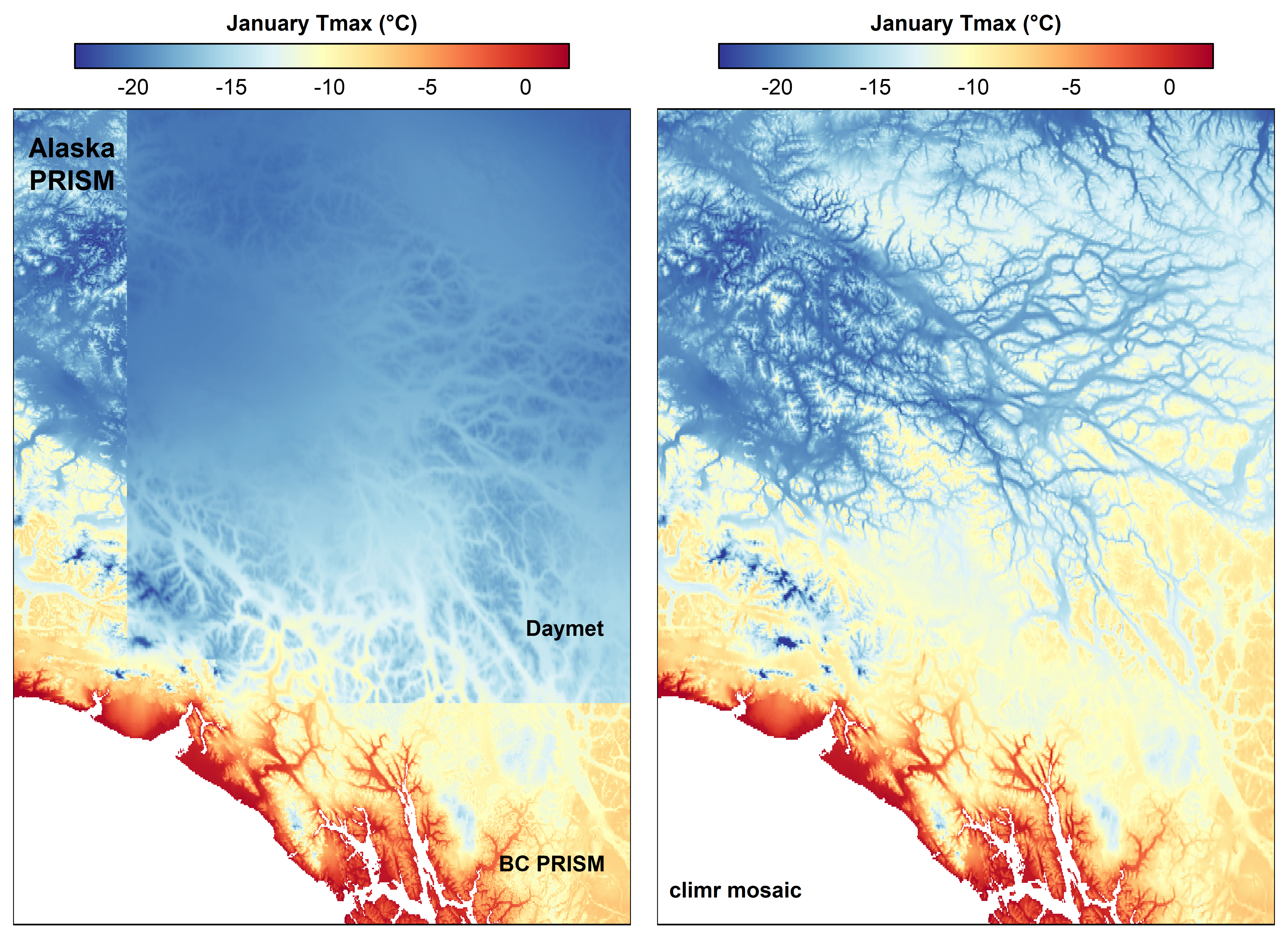
Figure 2. Source data and prediction of the PRISM emulator for January Tmax (i.e., monthly mean daily maximum temperature) in southwest Yukon.
Figure 3 provides further perspective on the PRISM emulator relative to other data sources, using January Tmin as an example. The ClimateNA mosaic (bottom panel) uses a blend of the BC PRISM with a legacy 1961-1990 4km Western Canadian PRISM for the Yukon. This degrades the BC PRISM in the 50km overlap region of northern BC and the differences in the two datasets confound cross-border analysis. The PRISM emulator (centre panel) produces a preferable mosaic, but it is not ideal. The centre of the image exhibits an abrupt, dubious transition from negative lapse rates (warm valleys, cold mountains) in BC to positive (inverted) lapse rates in the Yukon. This demonstrates the need for a more sophisticated PRISM emulation method. Further, it emphasizes that the PRISM emulator is not a substitute for the PRISM methodology.
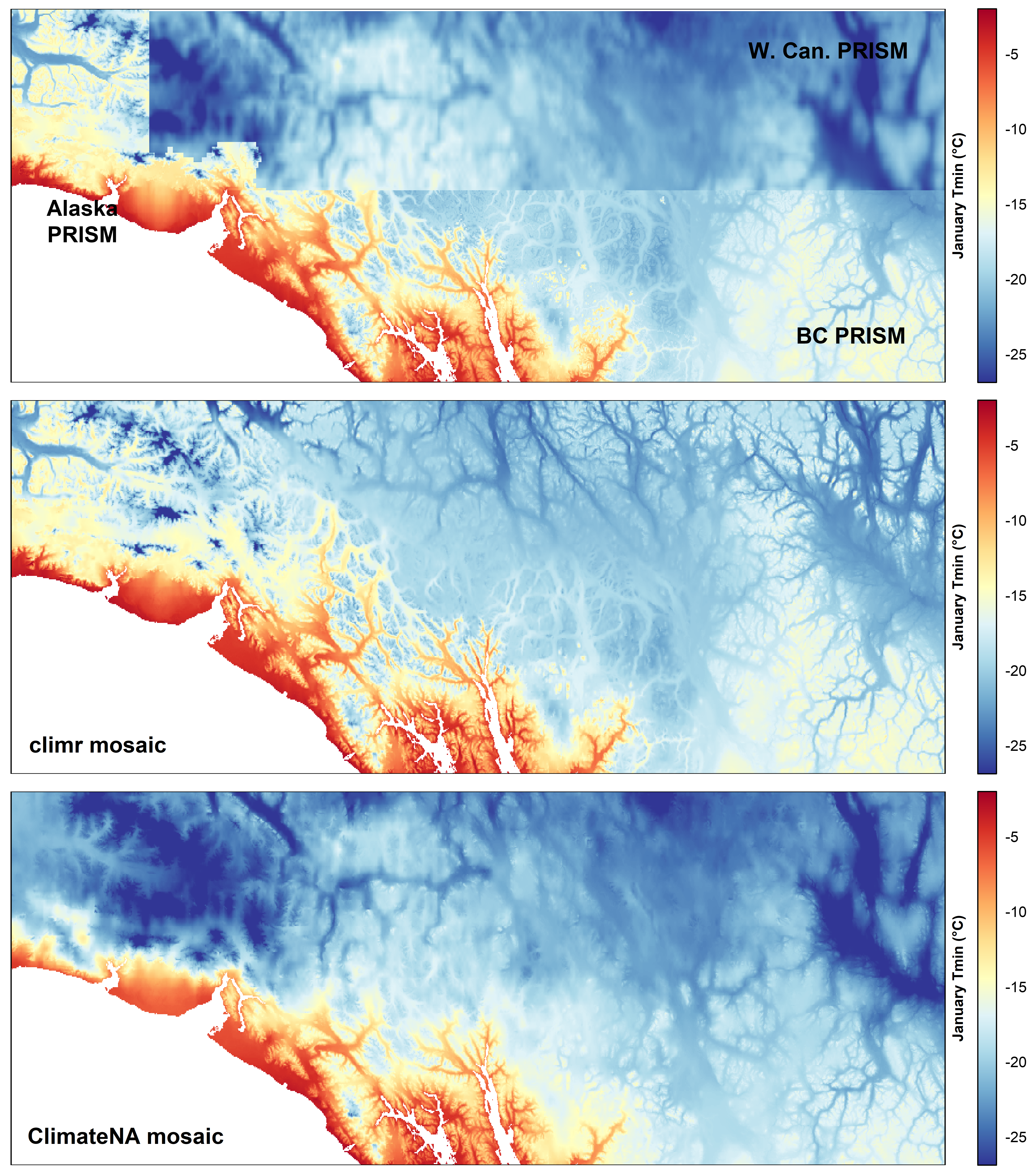
Figure 3. Comparison of climr and ClimateNA mosaics to source data for January Tmin in southwest Yukon.
BC-Alberta border
Figure 4 shows the results of the PRISM emulator along the BC-Alberta border at latitude 52-54.5oN. As in the Yukon, the PRISM emulator provides a credible extrapolation outside the BC border, avoding the need to blend an inferior map into the BC PRISM domain. Notably, ClimateNA is not able to recover spatial resolution through elevation adjustment, and the climatology of the Rocky Mountains is degraded as a result. The weather stations demonstrate the challenge of climate mapping in this region: Weather stations are exclusively at low elevations, providing little support for automatic lapse rate calculation used by WorldClim and Daymet. This emphasizes the necessity for expert-supervised climatological mapping methods such as PRISM.
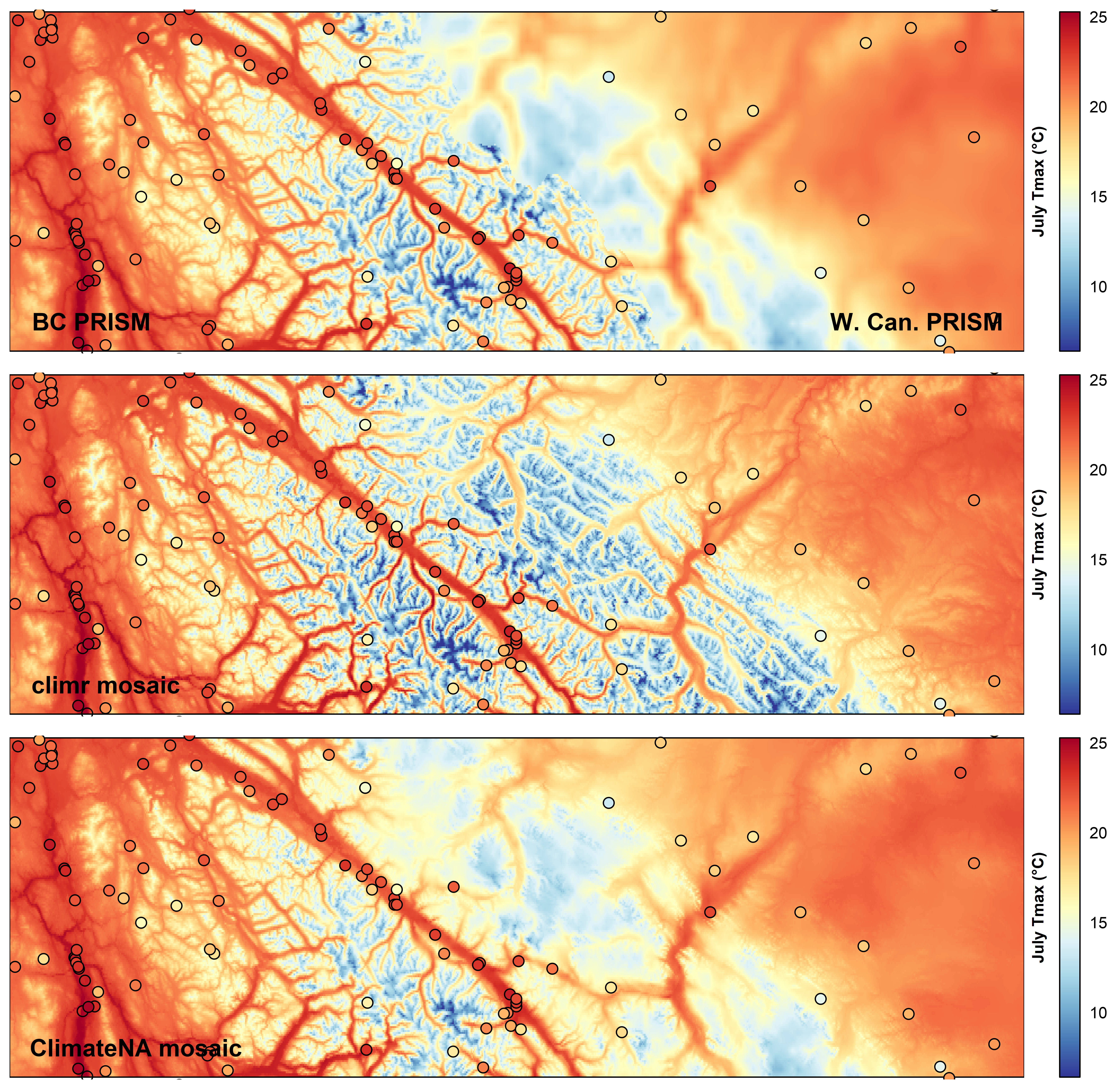
Figure 4. Comparison of climr and ClimateNA mosaics to source data for July Tmax at the continental divide boundary of southern BC and Alberta. Filled circles are weather stations with 1981-2010 normals following the same colour scheme.
BC-US border
The BC and US PRISM products are highly compatible for precipitation
and Tmax, and generally result in a seamless transition at the 49th
parallel Figure 5. Since precipitation is not
elevation-adjusted by default in climr, aggregating the climr mosaic to
2.5km resolution results in a blurring of the PRISM precipitation map
(Figure 5, center panel). We are not aware of observational or
theoretical evidence to support precipitation gradients at less than 3km
resolution in BC, except in dry valleys where virga (evaporation of
precipitation as it falls) could contribute to elevational gradients in
precipitation. As a result, this blurring in the climr mosaic likely is
generally acceptable. ClimateNA does apply elevation adjustment to
precipitation, as shown in the bottom panel of Figure 5, which results
in some valleys being drier than the original PRISM product. The climr
downscale() function provides an option for elevation
adjustment of precipitation (ppt_lr = TRUE) in both the
climr and ClimateNA mosaics.
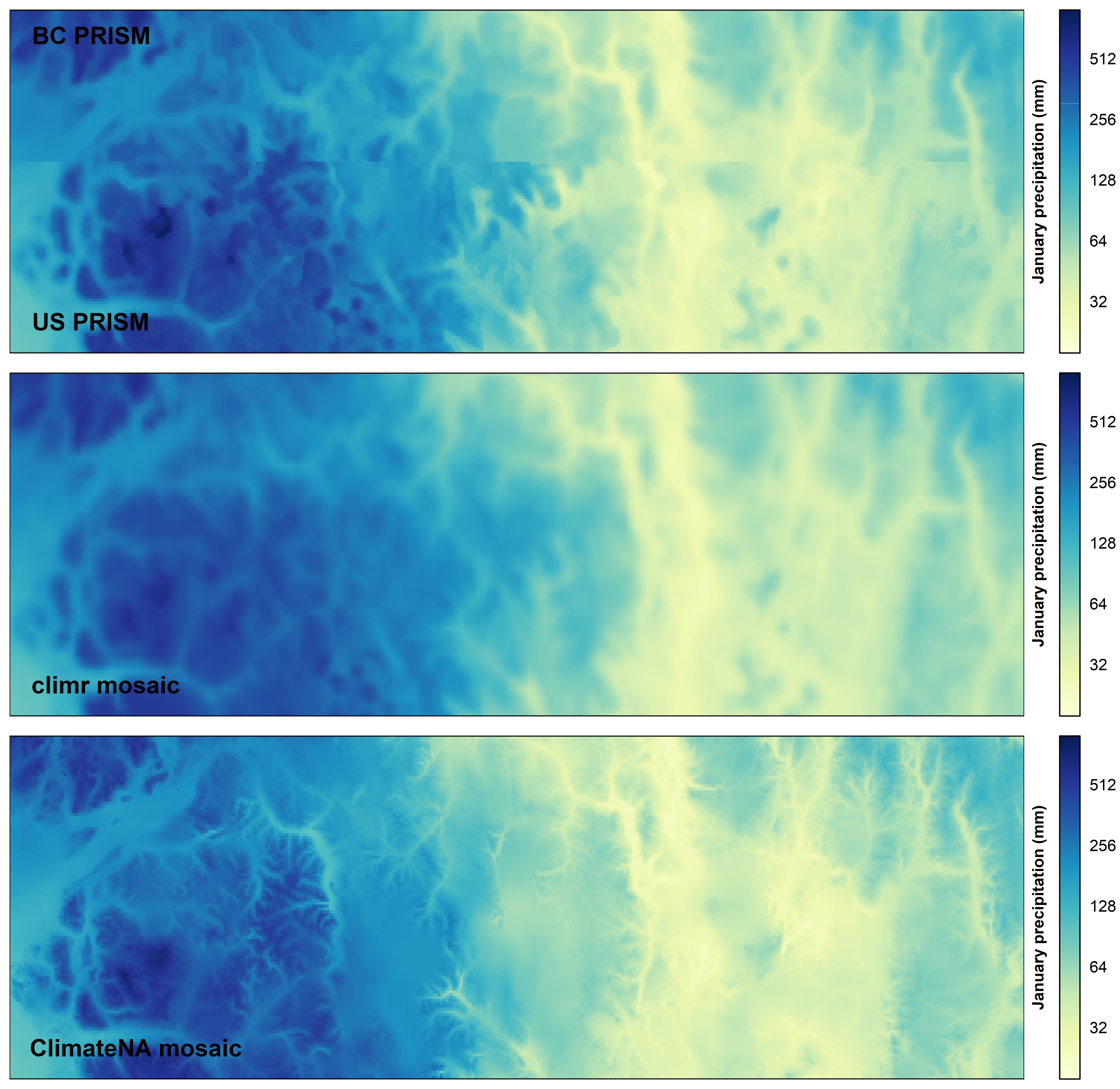
Figure 5. Comparison of climr and ClimateNA mosaics to source data for January precipitation along the boundary of southern BC and Washington State.
The BC and US PRISM products are significantly different for Tmin, as shown in Figure 6 (top panel) for January Tmin. The BC PRISM generally exhibits straightforward negative lapse rates (warm valleys, cold mountaintops), while the US PRISM exhibits a double reversal of elevational temperature gradients (warm-cool-warm-cool with elevation) in eastern and western portions of the image. This is likely an unintended artefact of the two-layer atmosphere technique employed in the US PRISM as a way of modeling the valley inversions (cold valleys, warm midslopes, cold mountaintops) that are common throughout the western United States. We investigate the evidence for the double-reversed lapse rates in the known issues section of this article. We did not find compelling evidence for these gradients based on a preliminary examination of station data, though further investigation would be required to rule them out.
Assuming that the double-reversed Tmin gradients are an artefact, some reduction in their prominence is desirable, and will contribute to more coherence between the BC and US components of the climr mosaic. Two aspects of the mosaic method contribute to a dampening of the Tmin gradients. First, the PRISM emulator was used to blend the BC and US PRISM between 48oN and 49oN. Second, the aggregation of the mosaic from 800m PRISM resolution to 2.5km resolution smooths the sharp gradient reversals. The recalculation of the climr mosaic at 800m resolution removes the gradient reversals, but does result in some regions with very low lapse rates (Figure 6, centre panel). This smoothing effect is more pronounced evident in the ClimateNA mosaic (Figure 6, bottom panel), where the 4km resolution of the ClimateNA mosaic results in loss of non-artefactual features such as the Columbia River valley and its tributaries at the far right of the image.
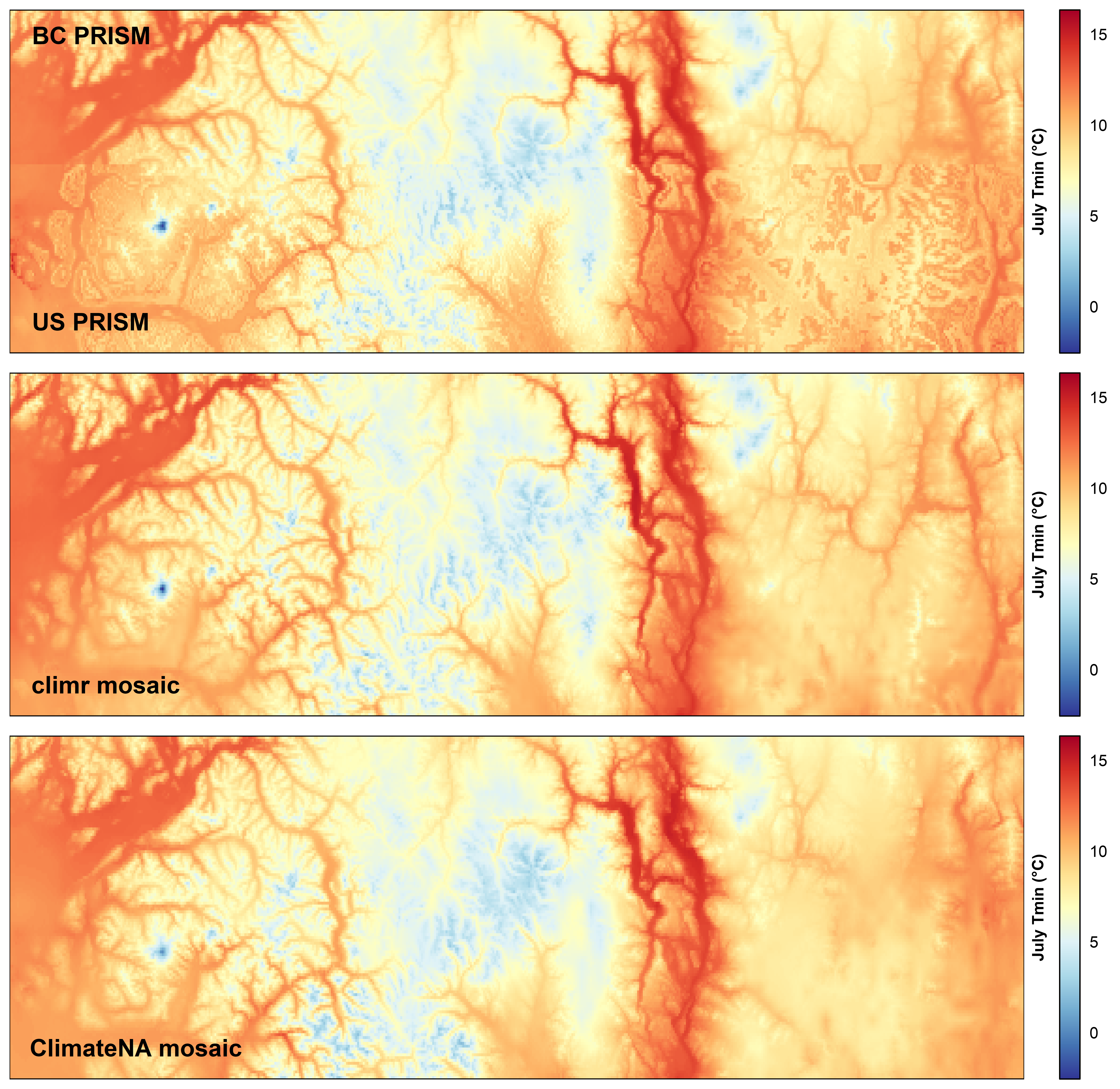
Figure 6. Comparison of climr and ClimateNA mosaics to source data for July Tmin along the boundary of southern BC and Washington State.
Alberta-US border
Daymet and PRISM precipitation have a different character over the prairies (Figure 7). PRISM precipitation is smooth, with blotches due to variability between weather stations. Daymet precipitation does not have obvious station artefacts, but has fine-scale features such as drier coulees/ravines that may or may not reflect reality (e.g., due to virga). To the extent that cross-border consistency is important to downstream analyses, it is beneficial to have a consistent product (Daymet) or method (PRISM) in the mosaic where possible. Providing both the ClimateNA and climr mosaics in climr gives users the option to select a product that best meets their needs.
The climr and ClimateNA mosaics both have an apparent discontinuity in January precipitation across the Canada-US Border. This discontinuity is also present in December and February. Since Daymet applies a consistent method across the border, this discontinuity is not simply a blending artefact. We have not yet established the reason for this effect and whether it is real.
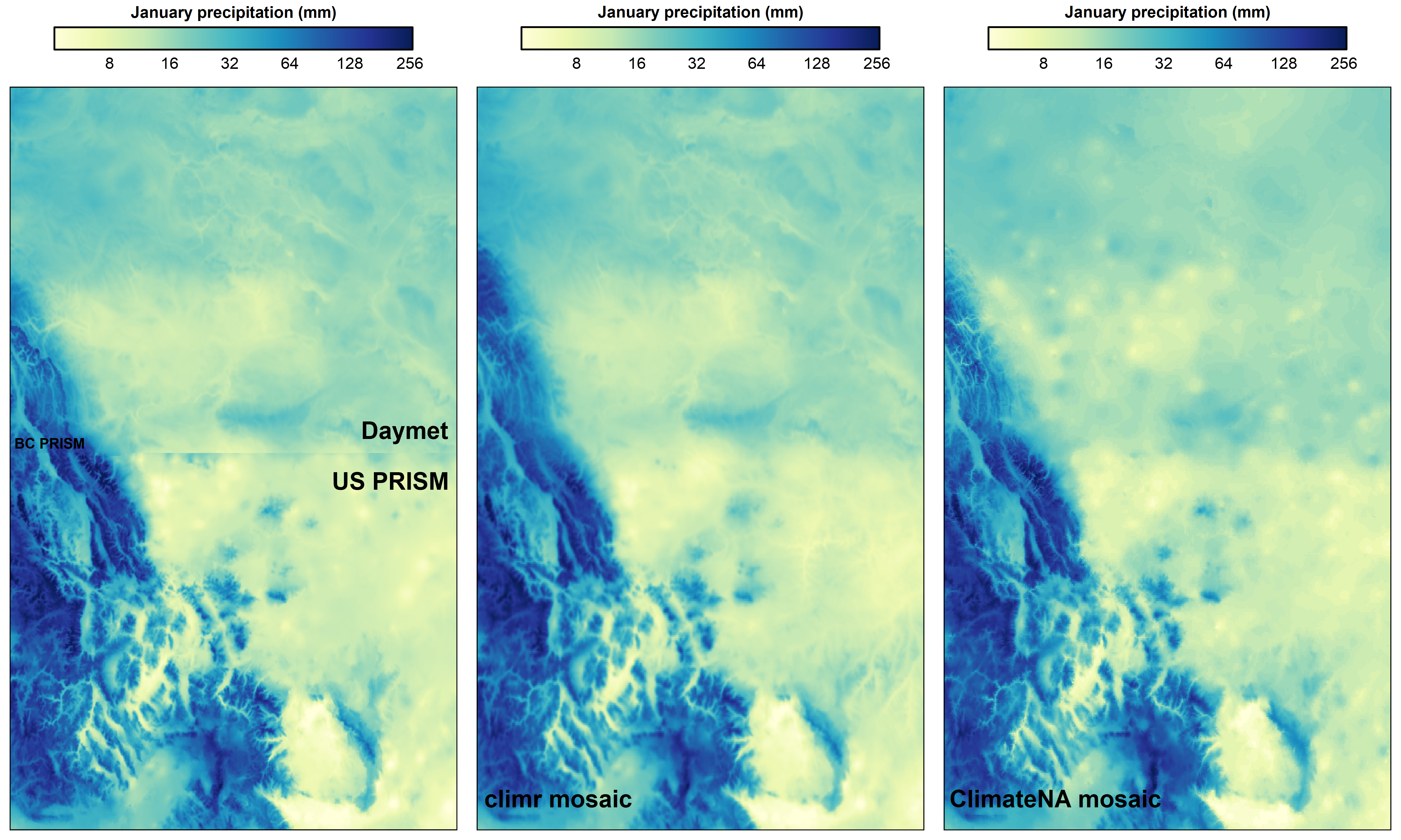
Figure 7. Comparison of climr and ClimateNA mosaics to source data for July Precipitation along the Alberta-US boundary.
US-Mexico border
Predictive blending is able to create a visually seamless transition from the US PRISM to Daymet over northwestern Mexico (Figure 8). The climatology of January precipitation in the climr mosaic is drier than in the ClimateNA mosaic along the west coast of mainland Mexico and in the Colorado river delta at the north end of the Gulf of California. We have not yet evaluated which is more consistent with station observations.
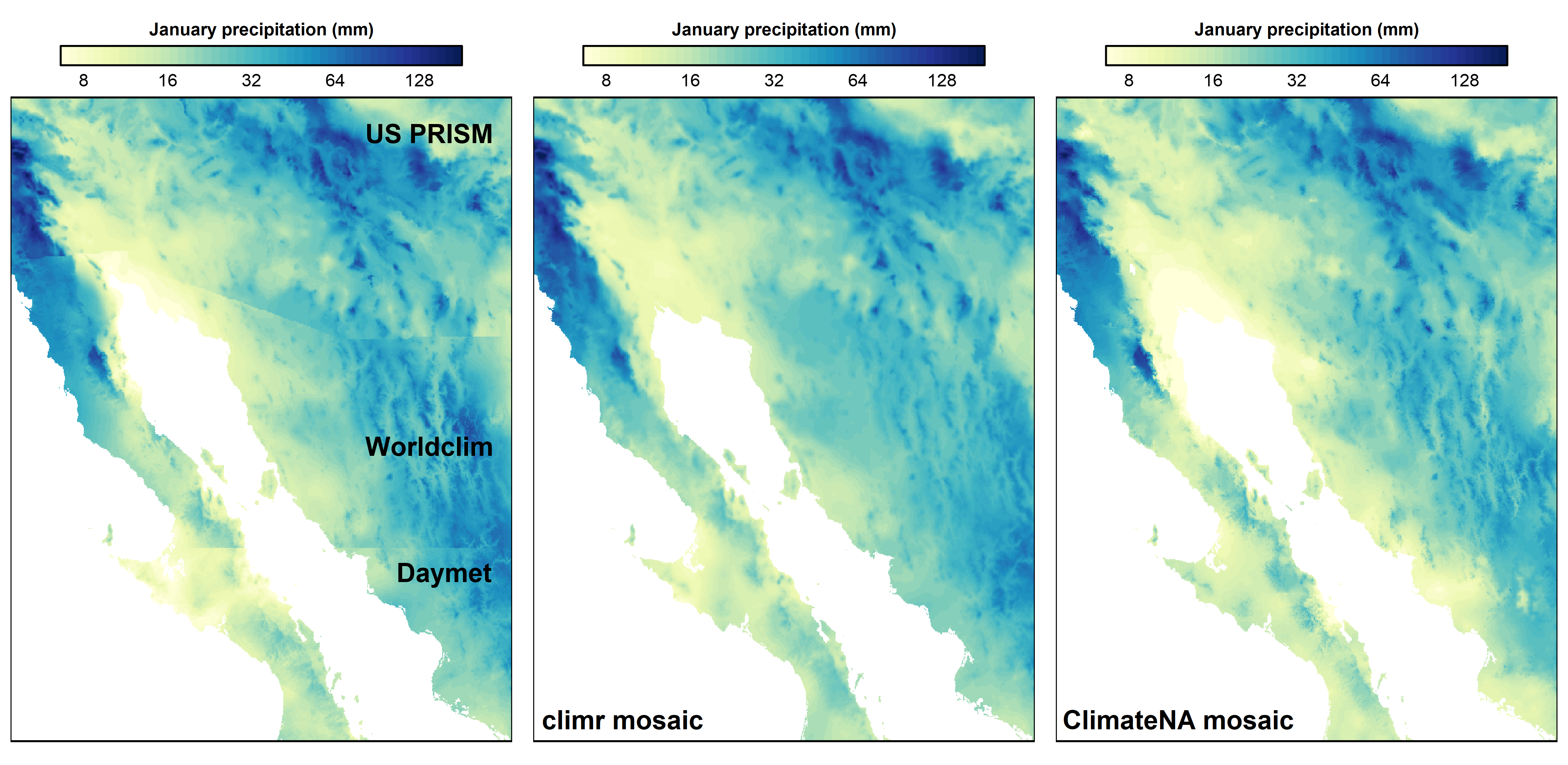
Figure 8. Comparison of climr and ClimateNA mosaics to source data for January Precipitation along the US-Mexico boundary.
Discussion and known Issues
Evaluation and refinement of the climr mosaic is ongoing. This section discusses known issues that require further work.
Double-reversed Tmin lapse rates in the US PRISM
As noted above, the US PRISM maps exhibit a double reversal of Tmin lapse rates (warm-cool-warm-cool with increasing elevation) in many regions of Montana, Idaho, and Washington State. This PRISM pattern may be an unintended artefact of PRISM’s two-layer atmosphere technique used to model valley inversions, in which different lapse rates are derived above and below an altitude of 250m above a regional base elevation (Daly et al. (2008)).
To investigate whether there is evidence for the double reversal, we compared elevation-Tmin relationships of station data and PRISM in four regions spanning the BC-US Border. The comparison for January Tmin is shown in Figure 9. In the West Kootenay region of BC (region 1), the station data strongly supports the monotonic negative lapse rate of ~-5oC/km employed by the BC PRISM. In the BC Rocky Mountains (Region 2), the station data is more ambiguous, and the BC PRISM uses a weaker monotonic lapse rate of ~-2oC/km in the southern portion of this region. South of the border in Washington State (Region 3), There are two groups of stations. Stations below 1100m elevation demonstrate a strong lapse rate of ~-5oC/km consistent with the Region 1 stations. The stations above 1100m are ambiguous. The US PRISM applies a strong lapse rate at these elevations (visible in the grey dots) requiring a double reversal of lapse rates. However, the station data as portrayed here would also be consistent with a weak lapse rate above 1100m, requiring no lapse rate reversals.
We investigated other months, and smaller subregions of regions 3 and 4, and found no compelling evidence for a double reversal of lapse rates. However, our analysis doesn’t account for topographic position of stations and other factors that could improve detection of complex lapse rates. Consequently, we can’t rule out the presence of double-reversed lapse rates.
Discussion with the developers of the US PRISM (Chris Daly, pers. comm., January 9, 2025) indicated three points: (1) a double reversal of lapse rates is possible, (2) the two-layer PRISM method can produce double-reversed temperature profiles as an artefact of sparse station data, and (3) definitive evidence for double-reversed temperature profiles is not available. Given this ambiguity, the simplification of the lapse rates that results from aggregating the climr mosaic to 2.5km seems justifiable. In absence of definitive evidence, the climr-modified lapse rates and the original PRISM can reasonably be considered as alternative interpretations of ambiguous station data.
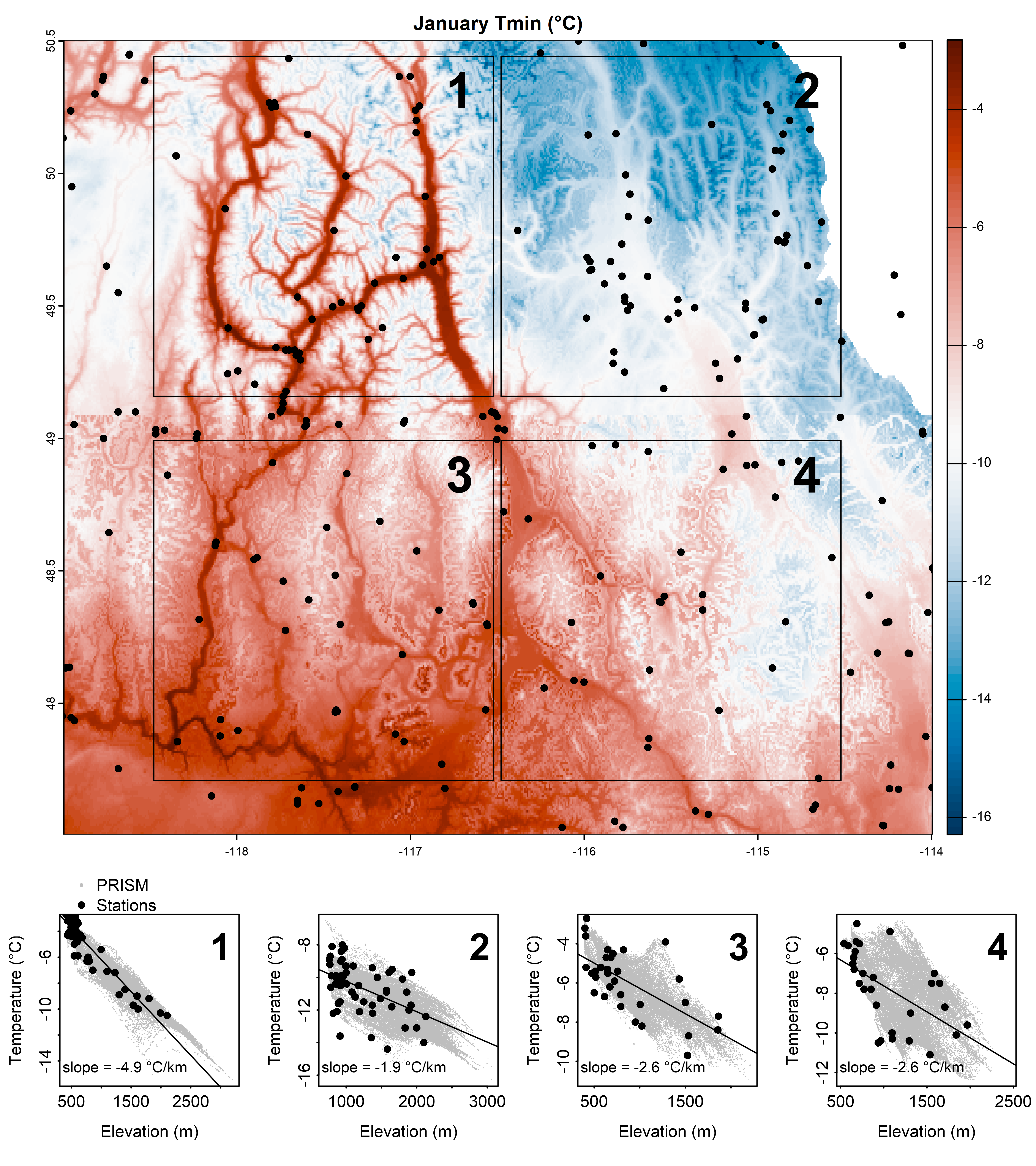
Figure 9. Evaluation of January Tmin lapse rates in the BC PRISM (areas 1 & 2) and US PRISM (areas 3 and 4). Black dots on the map are weather station locations. Bottom panels show the relationship of temperature to elevation in the PRISM grid cells (grey dots) and stations (black dots) within each of the four numbered square areas on the map. The line and stated slope are a linear best fit to the station data.
Extrapolation uncertainty in the PRISM emulator
The GAN models are trained on the PRISM climate map for BC and Alaska. Prediction into distant areas of the Yukon and Northwest Territories is an extrapolation subject to error associated with novel climate regimes. To estimate extrapolation uncertainty, we trained three GAN models each for March, June, October, and December. Since the models are stochastic, the intermodel variation likely is an indicator of novel conditions (combinations of predictor values such as topography and climate). In the example of June precipitation (Figure 10), there generally is very low intermodel variation in the training areas of BC and Alaska and high intermodel variation in the MacKenzie mountains. While we chose a single model prediction for the climr mosaic, this analysis of prediction variability indicates that there are spatially variable patterns of extrapolation error in the climr mosaic for Yukon and NWT. We intend to provide users with uncertainty maps in future versions of climr, and to refine our selection of GAN models to conserve the annual cycle of climatic variation at each location.
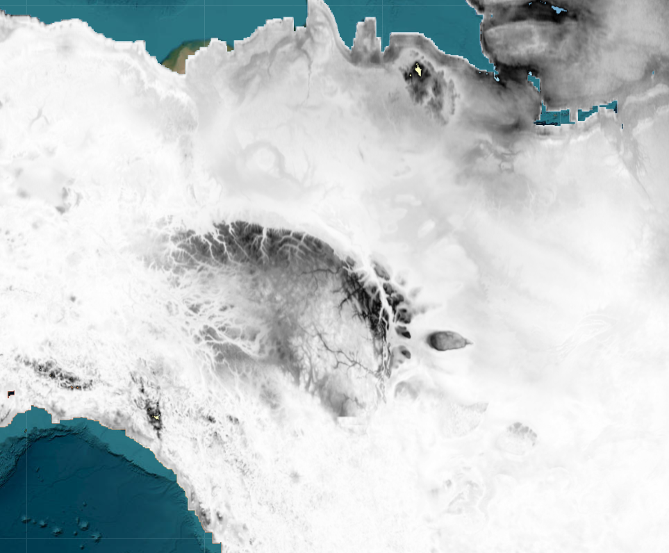
Figure 10. Standard deviation of June precipitation predictions from three deep learning models in the western arctic. Darker colors indicate higher variation among predictions, which likely is a proxy for prediction uncertainty.
Month-to-month consistency in the PRISM emulator
Our current PRISM emulation method uses a separate GAN model for each month of each climate element (e.g., January Tmin). Extrapolation errors are therefore not consistent across months. These temporal inconsistencies can produce artefacts in the seasonal cycle of each climate element at some locations (e.g., April colder than March) and unrealistic variation in lapse rates among adjacent months. While temporal inconsistencies are minor for temperature, they are more pronounced for precipitation. We are developing a more sophisticated method of PRISM emulation that provides temporal consistency between adjacent months, and will update the climr mosaic when possible. Until then, users should be corroborate the seasonal cycle of climr data with other evidence for their locations of interest in the Yukon and Northwest Territories.
Alberta foothills
The PRISM emulator for western Alberta is trained on the windward side of the Rocky Mountains (BC) and predicted onto the leeward side (Alberta). This raises the concern of extrapolation errors due to underestimation of processes such as continental air mass influence, rainshadow effects, and chinook winds. The prediction does incorporate Alberta climate (WorldClim) as a predictor, but given the sparsity of station data used by WorldClim this is unlikely to substantially mitigate extrapolation errors in most locations. We believe that the PRISM emulator is preferable to other products for most uses because of its cross-border compatibility and more realistic spatial detail. However, users should be aware that the climr mosaic for the Alberta foothills is poorly constrained by station data and is not yet validated. We are developing improved methods of PRISM emulation that will address these limitations.
Acknowledgements
We gratefully acknowledge the developers of the component climatologies in the climr mosaic, namely the Pacific Climate Impacts Consortium (British Columbia PRISM maps), the PRISM Climate Group (US PRISM maps), the NASA Oak Ridge National Laboratory (Daymet), and WorldClim.