Self-contained change-factor downscaling of observed and simulated climate data

downscale() provides downscaled climate variables for user-specified locations. It adapts a simple change-factor (aka "delta') downscaling approach originally implemented in ClimateNA. This approach downscales climate data in three stages:

Change-factor downscaling of coarse-resolution (50-200km grid) monthly temperature and precipitation data from climate models or observational sources to high-resolution (800m grid);
Elevation adjustment of temperature variables to provide scales finer than the high-resolution reference grid; and
Calculating derived variables from the downscaled monthly temperature and precipitation variables.

See vignette("methods_downscaling") for a description of the downscaling methodology.

downscale() is a user-friendly wrapper for downscale_core()

Usage

downscale(
  xyz,
  which_refmap = "auto",
  obs_periods = NULL,
  obs_years = NULL,
  obs_ts_dataset = NULL,
  gcms = NULL,
  ssps = NULL,
  gcm_periods = NULL,
  gcm_ssp_years = NULL,
  gcm_hist_years = NULL,
  max_run = 0L,
  cache = TRUE,
  ...
)

Arguments

xyz: a data.frame with the following columns "long", "lat", "elev", and a unique "id". Any extra columns will be ignored and not output.
which_refmap: character. Which map of 1961-1990 climatological normals to use as the high-resolution reference climate map for downscaling. Default is "auto", which selects, for each query point, the best available climatological normals map in declining order of "refmap_prism", "refmap_climr", and "refmap_climatena". Other options are one of list_refmaps(), which will provide a consistent reference map for all points.
obs_periods: character. Which historical period for observational climate data, averaged over this period. Options are list_obs_periods(). Default NULL
obs_years: integer. Vector of years to obtain individual years or time series of observational climate data. Default NULL. See list_obs_years() for available years.
obs_ts_dataset: character. The dataset to use for observational time series data. Options are "climatena" for the ClimateNA gridded time series or "cru.gpcc" for the combined Climatic Research Unit TS dataset (for temperature) and Global Precipitation Climatology Centre dataset (for precipitation). Defaults to NULL.
gcms: character. Vector of global climate model names. Options are list_gcms(). Defaults to NULL.
ssps: character. Vector of SSP-RCP scenarios (representative concentration pathways paired with shared socioeconomic pathways). Options are list_ssps(). Defaults to all scenarios available.
gcm_periods: character. 20-year reference periods for GCM simulations. Options are list_gcm_periods(). Defaults to NULL.
gcm_ssp_years: character. Timeseries years for GCM simulations of future scenarios specified by ssps. See list_gcm_ssp_years() for available years. Defaults to NULL.
gcm_hist_years: character. Timeseries years for GCM simulations of the historical scenario. See list_gcm_hist_years() for available years. Defaults to NULL.
max_run: integer. Maximum number of model runs to include. A value of 0 returns the ensembleMean only. Runs are included in the order they are found in the models data until max_run is reached. Defaults to 0L.
cache: logical. Cache data locally? Default TRUE
...: other arguments passed to downscale_core(). Namely: return_refperiod, vars, out_spatial and plot

Value

data.table of downscaled climate variables for each location. All outputs are returned in one table.

Details

downscale_core() parameters can be applied in downscale(). For example, setting ppt_lr = TRUE in downscale() will apply elevation adjustment to precipitation values.

Although which_refmap = "auto" is the default, users are cautioned that this can produce artefacts associated with downscaling to different reference climate maps within and outside the western North American boundary of refmap_climr. We recommend that queries spanning this boundary use which_refmap = "refmap_climatena".

Examples


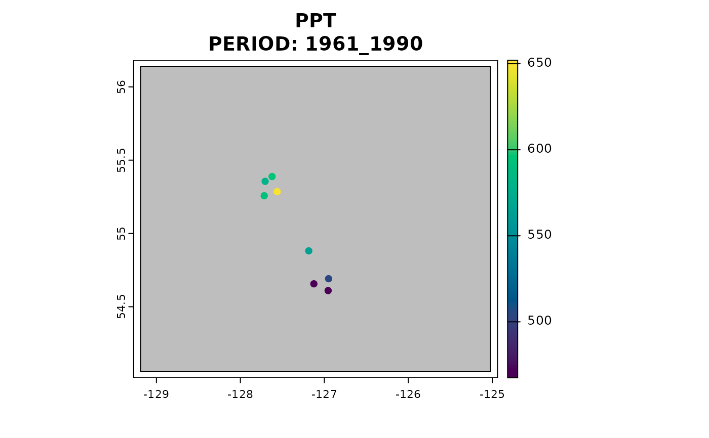
## provide or create a dataframe of lon, lat, elev, and id - usually read from csv file
in_xyz <- data.frame(
  lon = c(-127.7052, -127.6227, -127.5623, -127.7162, -127.1858, -127.125, -126.9495, -126.9550),
  lat = c(55.3557, 55.38847, 55.28537, 55.25721, 54.88135, 54.65636, 54.6913, 54.61025),
  elev = c(291, 296, 626, 377, 424, 591, 723, 633),
  id = 1:8
)

## historic observational time series
vars <- c("PPT", "CMD", "Tave_07")
climate_norms_hist <- downscale(
  xyz = in_xyz, 
  which_refmap = "auto",
  return_refperiod = TRUE,
  obs_periods = "2001_2020",
  vars = vars,
  out_spatial = TRUE, plot = "PPT"
) ## specify desired variables to plot
#> Welcome to climr!
#> 'gcms' is missing. 'max_run' will be ignored
#> Getting normals...
#> Downloading new data...
#> .
#> Caching data...
#> Getting observed anomalies...
#> Downloading observed period anomalies
#> .
#> Caching data...
#> Downscaling!!
#> Plotting results for a single period/GCM/run/SSP


## as a data.table
climate_norms_hist <- downscale(
  xyz = in_xyz, which_refmap = "auto",
  return_refperiod = TRUE,
  vars = vars,
  out_spatial = FALSE, plot = "PPT"
) ## specify desired variables to plot
#> Welcome to climr!
#> 'gcms' is missing. 'max_run' will be ignored
#> Getting normals...
#> Retrieving from cache...
#> Downscaling!!
#> Warning: 'gcms', 'gcm_ssp_ts', 'gcm_hist_ts', 'obs' and 'obs_ts' are missing. Nothing to downscale.

## future projections for annual variables from three models
climate_norms_fut <- downscale(
  xyz = in_xyz, which_refmap = "auto",
  gcms = list_gcms()[c(1,5,6)],
  ssps = list_ssps()[2],
  gcm_periods = list_gcm_periods()[1:2],
  # gcm_ssp_years = 2020:2060,
  max_run = 3, #' we want 3 individual runs for the model
  vars = list_vars("Annual")
)
#> Welcome to climr!
#> Getting normals...
#> Retrieving from cache...
#> Getting GCMs...
#> Downloading GCM anomalies
#> .
#> Caching data...
#> Downloading GCM anomalies
#> .
#> Caching data...
#> Downloading GCM anomalies
#> .
#> Caching data...
#> Downscaling!!