Intermediate `climr` workflow

Introduction

climr is in essence similar to ClimateNA in that it downscales low-resolution (~100km) global climate model anomalies to high-resolution (1-4km) maps of climate, with further elevation adjustment to user-specified elevation grids/points based on empirical lapse rates (local relationship of climate to elevation) of the 1-4km climate maps. The elevation-adjusted monthly values of basic climate elements (temperature and precipitation) are then used to estimate derived variables (e.g., degree-days, precipitation as snow) based on published equations and parameters from (Wang et al. 2016).

See vignette("methods_downscaling.Rmd") for a detailed explanation of the downscaling methodology employed in climr.

climr’s strengths are:

its ability to obtain multiple, individual runs of a (or several) General Circulation Model(s) (GCM), as well as the ensemble cross-run mean,

cloud-based raw data access and local data caching,
and direct R interface to downscaled climate elements and derived variables covering western Canada and western US.

In this vignette we cover two basic climr workflows to obtain historic and future climate projections of a few derived variables.

The first, less code-heavy, workflow uses downscale() to do much of the heavy lifting – [Workflow with downscale]. The second workflow is a step-by-step breakdown of downscale() using the functions downscale() calls internally – [Workflow with *_input functions and downscale].

Main functions

Below is a list of the main functions used in the two workflows.

downscale() takes a data.table of point coordinates (in lat-long projection), obtains climate normals and historic and/or future projections covering the extent of the points, which are then downscaled using point elevation data and used to calculate derived climate variables at the point locations. It outputs the downscaled and derived variables in the form of a data.table or SpatVector of points.
input_refmap() downloads and prepares high-resolution climate normals. Called internally by downscale().
input_obs() and input_obs_ts() download and prepare low-resolution historic climate elements for a given historic period or time series, respectively. Called internally by downscale().
input_gcms(), input_gcm_hist() and input_gcm_ssp() download and prepare low-resolution climate element projections for a future period, historic period or future time series, respectively. Called internally by downscale().
downscale() downscales historic or future climate elements and calculates derived climate variables. Called by downscale().

Workflow with `downscale`

In this example workflow we use downscale() to calculate mean annual temperature (MAT), total annual precipitation (PPT) and precipitation as snow (PAS) at weather stations associated with the Adjusted and homogenized Canadian climate data.

We will downscale MAT, PPT and MAS at these locations for a historic and a future period, using two separate runs of a GCM and one emissions scenario.

We begin by loading the Adjusted Precipitation for Canada (APC2) dataset and clipping it to the North Vancouver area. This dataset already contains elevation information.

Note that longitude (‘lon’) and latitude (‘lat’) must be in lat-long projection (EPSG:4326) and elevation in m. Point IDs must be unique – we will use the weather station IDs.

We will also add two other columns in our data.table (‘ZONE’ and ‘HEZ’) these are ignored by downscale(). downscale() preserves the IDs and we use them to join back the extra columns used for plotting later on.

library(climr)
library(data.table)
library(terra)

## weather station locations
weather_stations <- get(data("weather_stations")) |>
  unwrap()

## study area of interest (North Vancouver)
vancouver_poly <- get(data("vancouver_poly")) |>
  unwrap()

## subset to points in study area
weather_stations <- mask(weather_stations, vancouver_poly)

## convert to data.table and subset/rename columns needed by climr
xyzDT <- as.data.table(weather_stations, geom = "XY")
cols <- c("Station ID", "x", "y", "Elevation (m)")
xyzDT <- xyzDT[, ..cols]
setnames(xyzDT, c("id", "lon", "lat", "elev"))

## join BEC zones and colours
BECz_vancouver <- get(data("BECz_vancouver")) |>
  unwrap()

BECz_points <- extract(BECz_vancouver, weather_stations) |>
  as.data.table()
BECz_points <- BECz_points[, .(ZONE, HEX)]

xyzDT <- cbind(xyzDT, BECz_points)

## remove duplicates
xyzDT <- unique(xyzDT)

## there are some duplicate stations with slightly different
## coordinates. We'll take the first
xyzDT <- xyzDT[!duplicated(id)]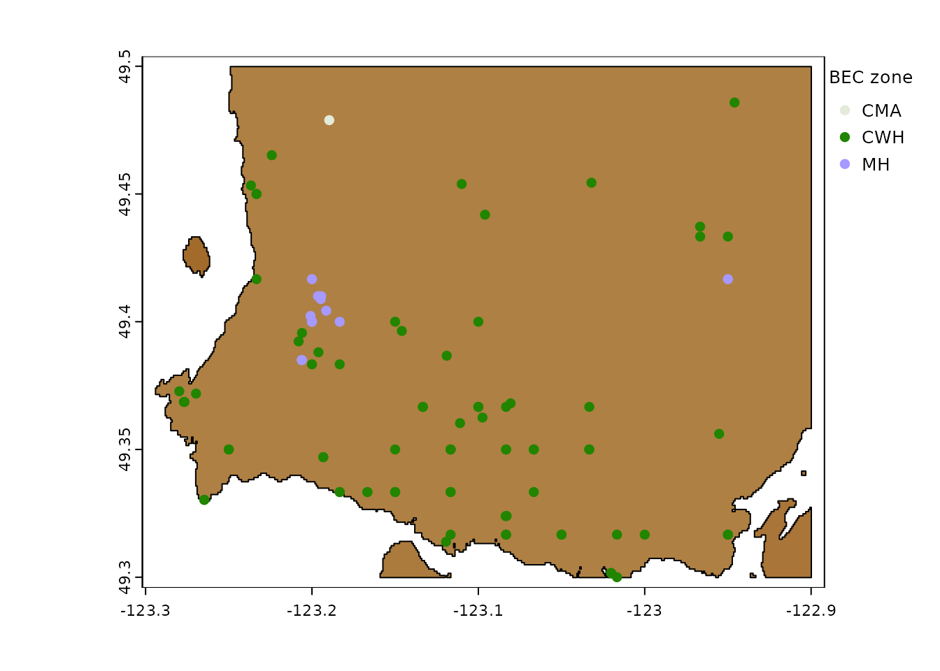

Weather stations in North Vancouver

The list_*() functions below provide a list of available historic and future periods, GCMs, emissions scenarios, and derived variables (in this case only the annual ones).

list_obs_periods()
#> [1] "2001_2020"

list_gcm_periods()
#> [1] "2001_2020" "2021_2040" "2041_2060" "2061_2080" "2081_2100"

list_gcms()
#>  [1] "ACCESS-ESM1-5" "BCC-CSM2-MR"   "CanESM5"       "CNRM-ESM2-1"  
#>  [5] "EC-Earth3"     "GFDL-ESM4"     "GISS-E2-1-G"   "INM-CM5-0"    
#>  [9] "IPSL-CM6A-LR"  "MIROC6"        "MPI-ESM1-2-HR" "MRI-ESM2-0"   
#> [13] "UKESM1-0-LL"

list_ssps()
#> [1] "ssp126" "ssp245" "ssp370" "ssp585"

list_vars(set = "Annual")
#>  [1] "AHM"     "bFFP"    "CMD"     "CMI"     "DD18"    "DD5"     "DDsub0" 
#>  [8] "DDsub18" "eFFP"    "EMT"     "Eref"    "EXT"     "FFP"     "MAP"    
#> [15] "MAT"     "MCMT"    "MSP"     "MWMT"    "NFFD"    "PAS"     "PPT"    
#> [22] "RH"      "SHM"     "Tave"    "TD"      "Tmax"    "Tmin"

We will chose the only available historic period (2001-2020), the 2021-2040 future period, the ‘EC-Earth3’ GCM and the SSP 2.45 scenario. MAT, PPT and PAS will be selected as output variables.

We pass our choices to downscale(), choosing the climr composite reference climatology (refmap_climr).

ds_out <- downscale(
  xyz = xyzDT,
  which_refmap = "refmap_climr",
  obs_periods = "2001_2020",
  gcm_periods = "2021_2040",
  gcms = "EC-Earth3",
  ssps = "ssp245",
  max_run = 2,
  return_refperiod = TRUE, ## to return the 1961-1990 normals period
  vars = c("MAT", "PPT", "PAS")
)
#> Welcome to climr!
#> Getting observed anomalies...
#> Downloading observed period anomalies
#> .
#> Caching data...
#> Getting GCMs...
#> Downloading GCM anomalies
#> .
#> Caching data...
#> Downloading new data from refmap_climr...
#> .
#> Caching data...
#> Downscaling...

Note how data from historical periods doesn’t have a GCM or SSP value – this is expected , as GCMs and SSPs are used to project future climate values. Also, future projections were obtained for two runs of EC-Earth3 (‘r1i1p1f1’ and ‘r10i1p1f1’), plus the ensemble mean.

‘ds_out’ table - Output from `downscale`. Outputs are show for one location (‘id’)
id	GCM	SSP	RUN	PERIOD	MAT	PPT	PAS
87	NA	NA	NA	1961_1990	10.31440	2652.915	90.61342
87	NA	NA	NA	2001_2020	11.15575	2641.369	62.38470
87	EC-Earth3	ssp245	ensembleMean	2021_2040	11.83280	2731.277	51.01070
87	EC-Earth3	ssp245	r15i1p1f1	2021_2040	11.39220	2821.350	64.38171
87	EC-Earth3	ssp245	r1i1p1f1	2021_2040	12.03708	2752.915	47.21344

To add back the extra columns we need only a simple left join.

ds_out <- xyzDT[, .(id, ZONE, HEX)][ds_out, on = .(id)]

We can now do a simple visualisation of climate variation by biogeoclimatic zone (‘ZONE’), in the normals period of 1961-1990:

plotdata <- melt(ds_out, measure.vars = c("MAT", "PPT", "PAS"))
cols <- plotdata$HEX
names(cols) <- plotdata$ZONE
cols <- cols[!duplicated(cols)]

ggplot(plotdata[PERIOD == "1961_1990"], aes(x = ZONE, y = value, fill = ZONE)) +
  geom_boxplot() +
  theme_light() +
  scale_fill_manual(values = cols) +
  facet_wrap(~variable, scales = "free")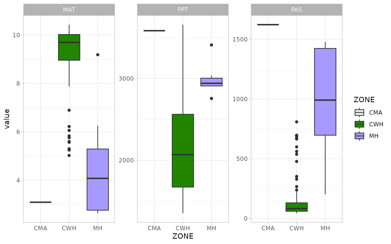

We may also want yearly climate projections. In this case, we want the yearly values of MAT and PPT for 2001-2015 and 2021:2040, using the same GCM, SSP and number of model runs. Notice how some of the data doesn’t need to be downloaded again, and was retrieved from cache.

The downscale() internally rescales the projected historical values so that they align with their observed counterpart. See vignette("methods_downscaling.Rmd") for details.

ds_out_ts <- downscale(
  xyz = xyzDT,
  obs_years = 2001:2023,
  gcm_hist_years = 2001:2014,
  gcm_ssp_years = 2015:2040,
  gcms = "EC-Earth3",
  ssps = "ssp245",
  max_run = 1,
  return_refperiod = TRUE, ## to return the 1961-1990 normals period
  vars = c("MAT", "PPT", "PAS")
)
#> Welcome to climr!
#> Downscaling in database...
#> Extracting [73] bands from refmap_climr
#> Extracting [624] bands from gcmts_VAR_ec-earth3
#> Extracting [1,008] bands from hist_ec-earth3

To plot the time series, we will filter the data to a single model run (i.e. in this case discard the ensemble means) and to a single point location. Note that we plot both the observed (obs_hist) and the projected historical (proj_hist) climate values along with future climate projections (proj_fut).

ds_out_ts[is.na(GCM), GCM := "Historic"]
ds_out_ts <- ds_out_ts[!grepl("ensemble", RUN)]
ds_out_ts <- ds_out_ts[!grepl("1961_1990", PERIOD)]

plotdata <- melt(ds_out_ts, measure.vars = c("MAT", "PPT", "PAS"))
plotdata[, PERIOD := as.numeric(PERIOD)]
plotdata <- plotdata[id == head(id, 1)]

## time series period groupings
plotdata[GCM == "Historic", pgrp := "obs_hist"]
plotdata[GCM != "Historic" & PERIOD <= 2020, pgrp := "proj_hist"]
plotdata[GCM != "Historic" & PERIOD > 2014, pgrp := "proj_fut"]

## make groups so that missing data is not shown as a "line connection"
groups <- data.table(PERIOD = unique(plotdata$PERIOD))
groups[, idx := c(1, diff(PERIOD))]
i2 <- c(1, which(groups$idx != 1), nrow(groups) + 1)
groups[, grp := rep(1:length(diff(i2)), diff(i2))]
plotdata <- groups[, .(PERIOD, grp)][plotdata, on = "PERIOD"]
plotdata[, grp := paste(grp, variable, sep = "_")]

yrbreaks <- c(
  min(plotdata$PERIOD),
  seq(min(plotdata$PERIOD), max(plotdata$PERIOD), by = 5),
  max(plotdata$PERIOD)
) |>
  unique()

ggplot(plotdata, aes(x = PERIOD, y = value, col = pgrp, group = grp)) +
  geom_line(
    data = plotdata[pgrp == "obs_hist"], size = 1.1,
    linejoin = "round", lineend = "round"
  ) +
  geom_line(
    data = plotdata[pgrp != "obs_hist"], size = 1.1,
    linejoin = "round", lineend = "round"
  ) +
  scale_x_continuous(breaks = yrbreaks, labels = yrbreaks) +
  scale_color_manual(
    values = c(
      "obs_hist" = "grey",
      "proj_hist" = "forestgreen",
      "proj_fut" = "navyblue"
    ),
    breaks = c("obs_hist", "proj_hist", "proj_fut")
  ) +
  theme_light() +
  theme(axis.text.x = element_text(angle = 45, vjust = 0.5)) +
  labs(x = "Year", col = "") +
  facet_wrap(~variable, scales = "free", ncol = 1, strip.position = "left", )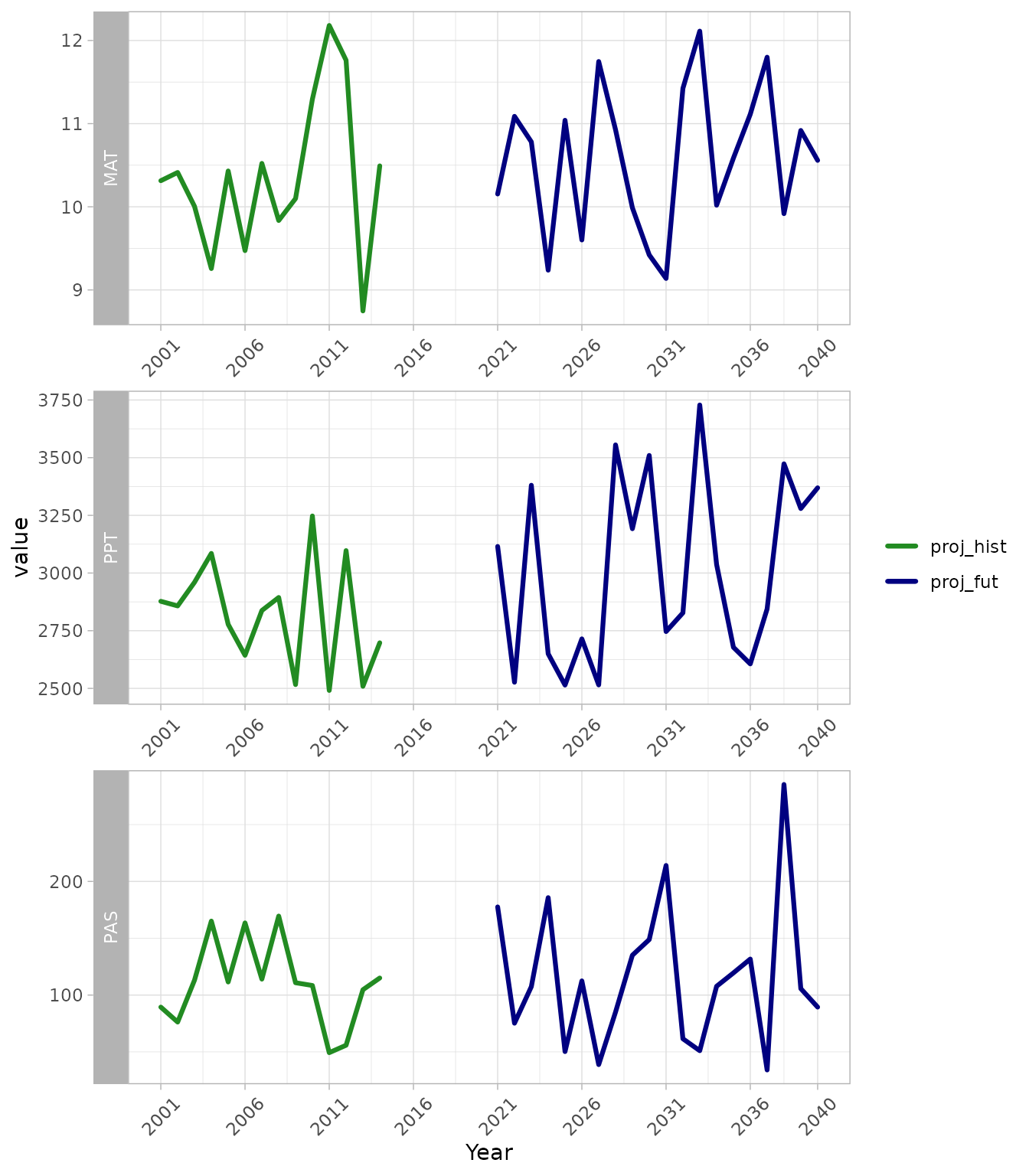

Time series outputs from downscale. Pannels show mean annual temperature (MAT), total annual precipitation (PPT) and precipitation as snow (PAS). Line colours refer to observed historic values (grey), projected historic values (gren) and future projected values (blue) for a single location, GCM, emissions scenario and model run.

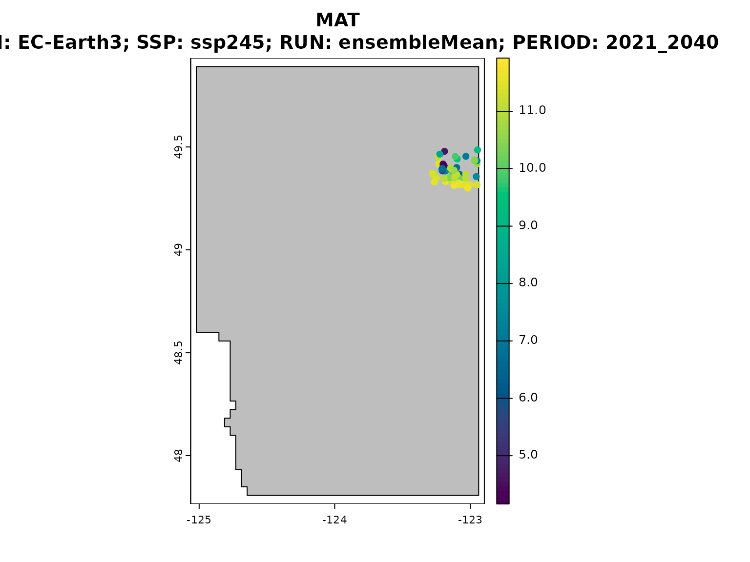
Spatial output and plotting options

downscale can also provide outputs in the form of a SpatVector of points and plot the values of a chosen climate variable from the list passed to downscale(..., vars), in this case MAT.

ds_out_spatial <- downscale(
  xyz = xyzDT,
  gcms = "EC-Earth3",
  gcm_periods = "2021_2040",
  ssps = "ssp245",
  max_run = 0,
  return_refperiod = FALSE, ## don't return the 1961-1990 normals period
  out_spatial = TRUE,
  plot = "MAT",
  vars = c("MAT", "PPT", "PAS")
)

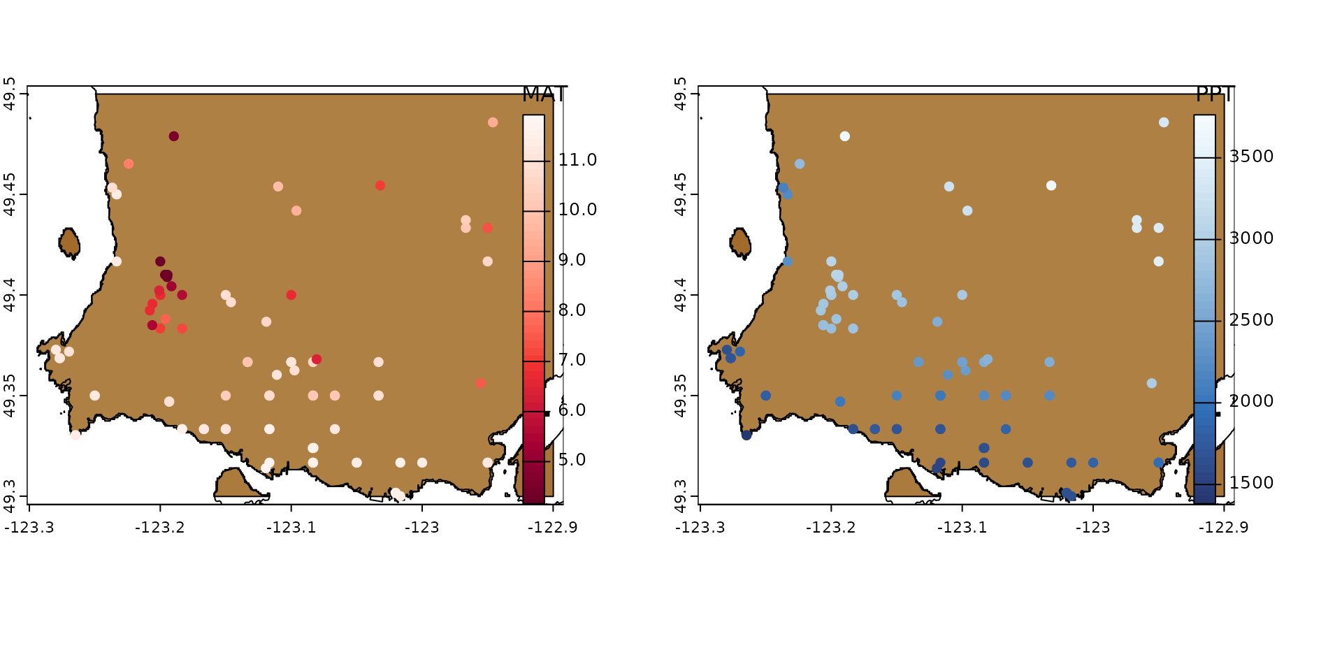
And of course we can now use the vector output to map all variables on top of our DEM raster, for prettier visuals:

vancouver <- get(data("vancouver")) |>
  unwrap()

par(mfrow = c(1, 2))
plot(vancouver_poly,
  col = hcl.colors(50, palette = "Earth"),
  plg = list(x = "bottom", title = "Elevation"),
  mar = c(4, 1, 1, 4)
)
plot(vancouver, add = TRUE, col = "black")
plot(ds_out_spatial, "MAT",
  col = hcl.colors(50, palette = "Reds"),
  add = TRUE, type = "continuous",
  plg = list(x = "right", title = "MAT")
)

plot(vancouver_poly,
  col = hcl.colors(50, palette = "Earth"),
  plg = list(x = "bottom", title = "Elevation"),
  mar = c(4, 1, 1, 4)
)
plot(vancouver, add = TRUE, col = "black")
plot(ds_out_spatial, "PPT",
  col = hcl.colors(50, palette = "Blues"),
  add = TRUE, type = "continuous",
  plg = list(x = "right", title = "PPT")
)

Workflow with `input_*` functions and `downscale_core()`

Alternatively, a user may choose to run the climate data preparation and downscaling functions separately.

We suggest doing this at least once or twice to have a full understanding of the steps that downscale executes internally.

Steps 1 and 2 bellow download and prepare the climate data used in the downscaling step (Step 3).

We will use the same point locations as above for downscaling.

1) Get climate normals - `input_refmap()`

When using input_refmap(), we establish a connection to the PostGIS server and pass the bounding box containing the point locations of interest.

There is no “auto” option to select the source of climate normals. list_refmap() provides a list of available options:

‘refmap_climatena’ corresponds to normals for North America obtained from ClimateNA (Wang et al. 2016);
‘refmap_climr’ corresponds to a composite of British Columbia PRISM, adjusted US PRISM and DAYMET (Alberta and Saskatchewan).

We will use ‘refmap_climr’ has it is the highest resolution product for the area of interest.

list_refmaps()
#> [1] "refmap_climr"     "refmap_climatena"

The extent of the downloaded climate anomalies will often be larger than the extent of the bounding box, and vary depending on the spatial resolution of the data. To demonstrate this we will define a bounding box with a set of coordinates.

Alternatively, get_bb could be used to extract bounding box around the point locations in xyzDT.

the_bb <- c(-124, -122, 49, 50)

normals <- input_refmap(
  bbox = the_bb,
  reference = "refmap_climr"
)
#> .

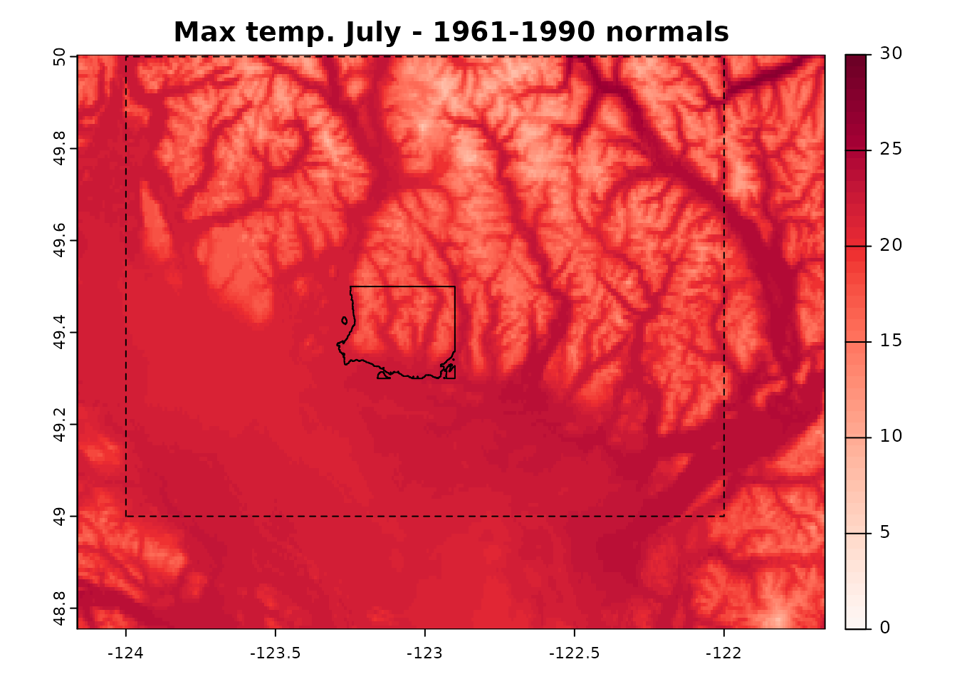
Downloaded normals shown with North Vancouver area and the requested bounding box.

2) Get climate projections and/or historical observations

Data for historic and future climate projections can be obtained with the gcm_*() functions. input_gcm_hist() is used to obtain historical anomalies projected with a (or several) GCM, whereas input_gcms() and input_gcm_ssp are used to obtain future anomaly projections for a period or individual years (i.e. time series).

Historical observations for a given period or for individual years can be obtained with input_obs and input_obs_ts, respectively.

hist_proj <- input_gcm_hist(
  bbox = the_bb,
  gcms = "EC-Earth3",
  years = 2001:2020,
  max_run = 0
)
#> .

fut_proj <- input_gcms(
  bbox = the_bb,
  gcms = "EC-Earth3",
  ssps = "ssp245",
  period = "2021_2040",
  max_run = 0
)
#> .

fut_proj_ts <- input_gcm_ssp(
  bbox = the_bb,
  gcms = "EC-Earth3",
  ssps = "ssp245",
  years = 2021:2040,
  max_run = 0
)
#> .

hist_obs <- input_obs(
  bbox = the_bb,
  period = "2001_2020"
)
hist_obs_ts <- input_obs_ts(
  bbox = the_bb,
  years = 2001:2020
)
#> .
#> .
#> .

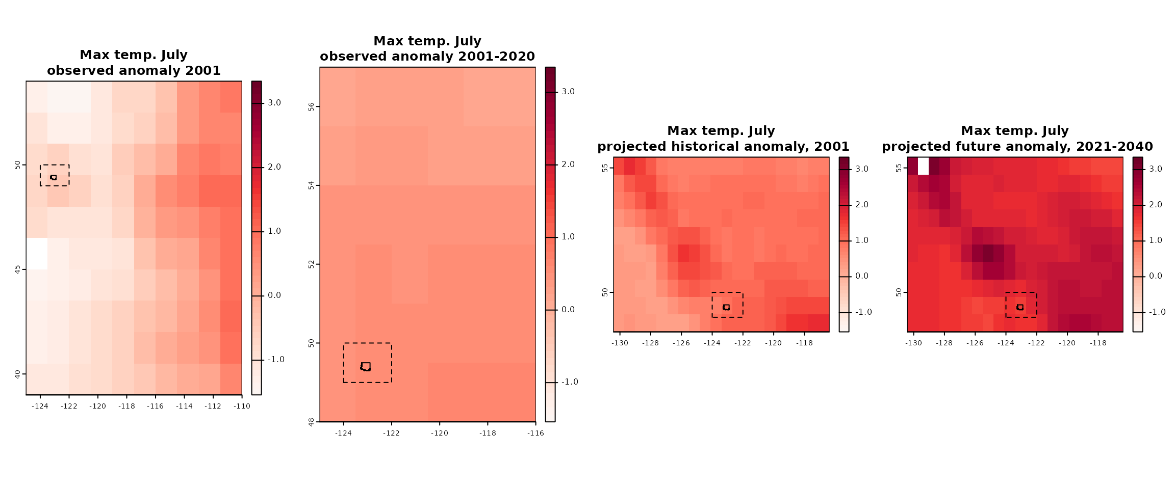
Downloaded historical and future anomalies shown with North Vancouver area and the requested bounding box.

3) Downscale and calculate actual values (i.e., not anomalies)

Now that we have all necessary inputs, we can downscale the climate data. To avoid repeating the same lines of code for each input, we’ll use lapply() and do.call() to iterate over the several climate inputs to downscale.

Note that for do.call() to work, our list of climate inputs (inputs) must be named according to downscale()’s argument names (you can list them with formalArgs(downscale)).



all_downscale <- downscale_core(xyzDT, refmap = normals, gcms = fut_proj, obs = hist_obs, gcm_ssp_ts = fut_proj_ts, gcm_hist_ts = hist_proj, obs_ts = hist_obs_ts, vars = "MAT", out_spatial = FALSE)
all_downscale

#> Key: <id, GCM, SSP, RUN, PERIOD, DATASET>
#>          id       GCM    SSP          RUN    PERIOD    DATASET      MAT
#>       <int>    <char> <char>       <char>    <char>     <char>    <num>
#>    1:    87      <NA>   <NA>         <NA> 1961_1990       <NA> 10.31440
#>    2:    87      <NA>   <NA>         <NA>      2001  climatena 10.72643
#>    3:    87      <NA>   <NA>         <NA>      2001   cru.gpcc 10.55995
#>    4:    87      <NA>   <NA>         <NA>      2001 mswx.blend 10.57633
#>    5:    87      <NA>   <NA>         <NA> 2001_2020       <NA> 11.15575
#>   ---                                                                  
#> 8532: 12936 EC-Earth3 ssp245 ensembleMean      2036       <NA> 12.12850
#> 8533: 12936 EC-Earth3 ssp245 ensembleMean      2037       <NA> 12.03018
#> 8534: 12936 EC-Earth3 ssp245 ensembleMean      2038       <NA> 11.73119
#> 8535: 12936 EC-Earth3 ssp245 ensembleMean      2039       <NA> 12.66107
#> 8536: 12936 EC-Earth3 ssp245 ensembleMean      2040       <NA> 11.86430

‘all_downscale’ table after binding. Outputs are shown for one location (‘id’)
id	GCM	SSP	RUN	PERIOD	DATASET	MAT
87	NA	NA	NA	1961_1990	NA	10.31440
87	NA	NA	NA	2001	climatena	10.72643
87	NA	NA	NA	2001	cru.gpcc	10.55995
87	NA	NA	NA	2001	mswx.blend	10.57633
87	NA	NA	NA	2001_2020	NA	11.15575
87	NA	NA	NA	2002	climatena	10.86645
87	NA	NA	NA	2002	cru.gpcc	10.61206
87	NA	NA	NA	2002	mswx.blend	10.65957
87	NA	NA	NA	2003	climatena	11.36302
87	NA	NA	NA	2003	cru.gpcc	11.21596
87	NA	NA	NA	2003	mswx.blend	11.16774
87	NA	NA	NA	2004	climatena	11.85929
87	NA	NA	NA	2004	cru.gpcc	11.59195
87	NA	NA	NA	2004	mswx.blend	11.68892
87	NA	NA	NA	2005	climatena	11.43069
87	NA	NA	NA	2005	cru.gpcc	11.11371
87	NA	NA	NA	2005	mswx.blend	11.13827
87	NA	NA	NA	2006	climatena	11.22500
87	NA	NA	NA	2006	cru.gpcc	11.10570
87	NA	NA	NA	2006	mswx.blend	11.14185
87	NA	NA	NA	2007	climatena	10.64902
87	NA	NA	NA	2007	cru.gpcc	10.59266
87	NA	NA	NA	2007	mswx.blend	10.55555
87	NA	NA	NA	2008	climatena	10.31697
87	NA	NA	NA	2008	cru.gpcc	10.15291
87	NA	NA	NA	2008	mswx.blend	10.19360
87	NA	NA	NA	2009	climatena	10.76312
87	NA	NA	NA	2009	cru.gpcc	10.40095
87	NA	NA	NA	2009	mswx.blend	10.67064
87	NA	NA	NA	2010	climatena	11.24732
87	NA	NA	NA	2010	cru.gpcc	11.02224
87	NA	NA	NA	2010	mswx.blend	11.12937
87	NA	NA	NA	2011	climatena	10.14367
87	NA	NA	NA	2011	cru.gpcc	10.05212
87	NA	NA	NA	2011	mswx.blend	10.06136
87	NA	NA	NA	2012	climatena	10.71056
87	NA	NA	NA	2012	cru.gpcc	10.50762
87	NA	NA	NA	2012	mswx.blend	10.65522
87	NA	NA	NA	2013	climatena	11.26619
87	NA	NA	NA	2013	cru.gpcc	11.14404
87	NA	NA	NA	2013	mswx.blend	11.06804
87	NA	NA	NA	2014	climatena	11.74145
87	NA	NA	NA	2014	cru.gpcc	11.50996
87	NA	NA	NA	2014	mswx.blend	11.55710
87	NA	NA	NA	2015	climatena	12.46339
87	NA	NA	NA	2015	cru.gpcc	12.14612
87	NA	NA	NA	2015	mswx.blend	12.38760
87	NA	NA	NA	2016	climatena	11.93472
87	NA	NA	NA	2016	cru.gpcc	11.80383
87	NA	NA	NA	2016	mswx.blend	11.88555
87	NA	NA	NA	2017	climatena	11.09313
87	NA	NA	NA	2017	cru.gpcc	10.71589
87	NA	NA	NA	2017	mswx.blend	10.94109
87	NA	NA	NA	2018	climatena	11.55876
87	NA	NA	NA	2018	cru.gpcc	11.14928
87	NA	NA	NA	2018	mswx.blend	11.62706
87	NA	NA	NA	2019	climatena	11.31839
87	NA	NA	NA	2019	cru.gpcc	10.68533
87	NA	NA	NA	2019	mswx.blend	11.15299
87	NA	NA	NA	2020	climatena	11.32559
87	NA	NA	NA	2020	cru.gpcc	11.11741
87	NA	NA	NA	2020	mswx.blend	11.21679
87	EC-Earth3	NA	ensembleMean	2001	NA	10.95358
87	EC-Earth3	NA	ensembleMean	2002	NA	10.99497
87	EC-Earth3	NA	ensembleMean	2003	NA	11.51956
87	EC-Earth3	NA	ensembleMean	2004	NA	11.28997
87	EC-Earth3	NA	ensembleMean	2005	NA	11.50313
87	EC-Earth3	NA	ensembleMean	2006	NA	10.84183
87	EC-Earth3	NA	ensembleMean	2007	NA	11.28038
87	EC-Earth3	NA	ensembleMean	2008	NA	10.87563
87	EC-Earth3	NA	ensembleMean	2009	NA	10.98315
87	EC-Earth3	NA	ensembleMean	2010	NA	11.94478
87	EC-Earth3	NA	ensembleMean	2011	NA	12.05804
87	EC-Earth3	NA	ensembleMean	2012	NA	11.29026
87	EC-Earth3	NA	ensembleMean	2013	NA	10.83139
87	EC-Earth3	NA	ensembleMean	2014	NA	11.56841
87	EC-Earth3	ssp245	ensembleMean	2021	NA	11.55924
87	EC-Earth3	ssp245	ensembleMean	2021_2040	NA	11.81754
87	EC-Earth3	ssp245	ensembleMean	2022	NA	12.10873
87	EC-Earth3	ssp245	ensembleMean	2023	NA	11.63212
87	EC-Earth3	ssp245	ensembleMean	2024	NA	11.36052
87	EC-Earth3	ssp245	ensembleMean	2025	NA	11.89326
87	EC-Earth3	ssp245	ensembleMean	2026	NA	11.81975
87	EC-Earth3	ssp245	ensembleMean	2027	NA	12.23477
87	EC-Earth3	ssp245	ensembleMean	2028	NA	11.82740
87	EC-Earth3	ssp245	ensembleMean	2029	NA	11.59876
87	EC-Earth3	ssp245	ensembleMean	2030	NA	11.69573
87	EC-Earth3	ssp245	ensembleMean	2031	NA	11.43653
87	EC-Earth3	ssp245	ensembleMean	2032	NA	12.24461
87	EC-Earth3	ssp245	ensembleMean	2033	NA	12.13565
87	EC-Earth3	ssp245	ensembleMean	2034	NA	11.28373
87	EC-Earth3	ssp245	ensembleMean	2035	NA	11.92043
87	EC-Earth3	ssp245	ensembleMean	2036	NA	11.96734
87	EC-Earth3	ssp245	ensembleMean	2037	NA	11.87066
87	EC-Earth3	ssp245	ensembleMean	2038	NA	11.56028
87	EC-Earth3	ssp245	ensembleMean	2039	NA	12.50379
87	EC-Earth3	ssp245	ensembleMean	2040	NA	11.69759

References

Wang, Tongli, Andreas Hamann, Dave Spittlehouse, and Carlos Carroll. 2016. “Locally Downscaled and Spatially Customizable Climate Data for Historical and Future Periods for North America.” Edited by Inés Álvarez. PLOS ONE 11 (6): e0156720. https://doi.org/10.1371/journal.pone.0156720.