Global climate model ensemble selection
methods_ensembleSelection.RmdSelection of the global climate model ensemble
The 13 global climate models available in climr were selected by Mahony et al. (2022) using the following criteria:
Criterion 1: Minimum of 3 historical runs available. This criterion ensures robust bias correction. Bias correction in climr is performed using the delta method: in which each model’s simulations are adjusted to remove the difference (delta factor) between the simulated and observed climate during the 1961-1990 reference period. Calculating the delta factor from the mean of at least three simulations reduces the confounding influence of the internal variability of individual runs on bias correction. 44 ScenarioMIP models passed this criterion.
Criterion 2: Tmin and Tmax
available. Tmin and Tmax are basic
climate variables for climr. Any models that do not provide
these variables are incompatible with climr. 10 models
failed this criterion. Notably, CESM2 does provide Tmin and
Tmax in their future projections, but due to an archiving
error these variables are not available for the historical runs of this
model.
Criterion 3. Complete scenarios. Models need to have at least one simulation of each of the four major SSP marker scenarios (SSP1-2.6, SSP2-4.5, SSP3-7.0, and SSP5-8.5). eight models failed this criterion.
Criterion 4. One model per institution. This criterion is a widely applied best practice in ensemble selection (Leduc et al. 2016). The rationale for each selection is provided below.
CNRM-ESM2-1 (ECS 4.8oC) was chosen over CNRM-CM6-1 (ECS 4.9oC) to give preference to the ESM over the AOGCM configuration;
EC-Earth3 (ECS 4.3oC) was arbitrarily chosen over EC-Earth3-Veg (ECS 4.3oC);
INM-CM5-0 (ECS 1.9oC) was arbitrarily chosen over INM-CM4-8 (ECS 1.8oC);
MPI-ESM1-2-HR (ECS 3.0oC) was chosen over MPI-ESM1-2-LR (ECS 3.0oC) due to its high resolution and availability of >1 run for all but SSP5-8.5.
MIROC6 (ECS 2.6oC) was chosen over MIROC-ES2L (ECS 2.7oC) because it has more runs/scenario, higher resolution, and because the latter has very high temperature bias over British Columbia.
For the purposes of this ensemble, different physics or forcing schemes were considered different models. We used only the r*i1p3f1 variants of the GISS-E2-1-G model, as these had the most complete set of scenario simulations.
Criterion 5. No closely related models. Models that share components were excluded, following Figure 5 of Brunner et al. (2020). NESM3 was excluded due to its close relation to MPI-ESM1.
Criterion 6. No large biases. Bias correction as performed in climr disrupts the physical connection between climate variables, and these distortions increase with the size of the biases in the simulation. For this reason, models with small biases are preferable to models with large biases, all else being equal. In an assessment over British Columbia, the AWI-CM-1-1-MR showed extreme temperature biases that warranted exclusion from the ensemble.
The 13-model ensemble has a mean global equilibrium climate sensitivity (ECS) of 3.7oC and a range of 1.9-5.6oC, which matches the full CMIP6 ensemble ECS (3.7oC; 1.8-5.6oC, Meehl et al. 2020.
The 8-model ensemble recommended for general purpose
All 13 models provided in climr are valid for analysis relative to warming levels. However, Mahony et al. (2022) recommended a subset of 8 models for ensemble analysis, based on the following four criteria:
Criterion 7. Constraints on equilibrium climate sensitivity (ECS). Multiple lines of evidence indicate that the Earth’s equilibrium climate sensitivity (ECS) is very likely between 2oC and 5oC (Hausfather et al. 2022). The evidence for the lower bound is robust, and weaker for the upper bound. From one perspective, inclusion of models with ECS outside this range uneccessarily increases the modeling uncertainty in downstream analyses. The opposing perspective is that high-sensitivity models are useful as a representation of high-impact, low-likelihood scenarios (Sutton and Hawkins 2020). Both perspectives are valid, and the preference depends on the objectives of each analysis.
Criterion 8. Model resolution. Four of the climr models are high enough resolution to resolve macrotopography e.g., to clearly differentiate the coast mountains from the Columbia/Rocky Mountains. This resolved macrotopography does produce elevation-dependent climate change signals and rainshadow effects. These models are weighted towards inclusion despite other criteria such as a low number of simulations per scenario. Conversely, models with very low resolution are weighted towards exclusion.
Criterion 9. Number of simulation runs. climr is primarily designed for analysis of projected climate normals; the climate change signal is of primary interest. Internal variability of the models are a confounding factor, producing erratic climate change trajectories in noisy climate variables like precipitation and winter temperature. The signal-to-noise ratio is increased by averaging the projected normals over multiple simulations of the same emissions scenario. Four models (BCC, INM, GFDL, and MRI) have only one run for most of the four scenarios, and this is a consideration for their exclusion.
Criterion 10: Spatial pattern. IPSL-CM6A-LR has a
pronounced pattern of localized summer heating along the BC coast
ranges, and little warming in some adjacent cells. This pattern is
present for both Tmin and Tmax for all summer
months. This may be a physically credible response within the model
context, for example due to a snow albedo feedback. However, for the
purposes of climr it would be problematic to downscale this
warming pattern across all elevations within the cell. This problem is
not isolated to IPSL-CM6A-LR, but the cell-to-cell contrast is
especially pronounced in IPSL and could create artefacts for analyses
based on climr.
The following models are excluded based on the combination of the four screening criteria:
CanESM5, because its very low horizontal resolution creates grid-box artefacts in downscaling and because its very high climate sensitivity (ECS 5.6oC) is also represented by UKESM1-0-LL.
INM-CM5-0, because it has very low climate sensitivity (ECS 1.9oC) and is an outlier among CMIP6 models for under-representing the observed 1975-2014 global temperature trend (Liang et al. 2020). In addition, this model has only one simulation for most scenarios, producing a less robust climate signal.
BCC-CSM2-MR, due to having a single simulation for each scenario and very low topographic resolution.
IPSL-CM6A-LR, due to isolated grid cells with very high summer warming in the BC Coast Ranges. The warming in these cells may be physically plausible (e.g., due to snow albedo feedbacks) in the model’s simplified topography, but is problematic for downscaling to high spatial resolution in climr.
A fifth model, UKESM1-0-LL, also has very high climate sensitivity, similar to CanESM5, that is assessed as very unlikely based on observational evidence. Some researchers may wish to constrain their analysis ensemble to observations by excluding this model. Others may wish to include this model in their ensembles as a representation of the long tail of uncertainty in the upper limit of climate sensitivity (Sutton 2018).
The 8-model subset that excludes UKESM1-0 has a mean global ECS of 3.4oC (2.6-4.8oC).
Comparison of the 13-model and 8-model ensemble
The differences between the 13-model and 8-model ensembles are illustrated in Figure 1. For mean summer daily maximum temperature (tasmax/Tmax_sm) averaged over North America, the 13-model ensemble mean is 0.5oC (13%) warmer than the 8-model ensemble mean. The proportional differences are greater in higher emissions scenarios (Figure 1, top). The difference between the ensembles is roughly equal to the difference between adjacent scenarios in mid-century (2040-2070), but is less important than differences among scenarios later in the century. This emphasizes that uncertainty in future emissions overshadows the differences between the 13-model and 8-model ensemble means.
The range of year-to-year variability is much greater in the 13-model ensemble (Figure 1, bottom). This is largely due to the extreme warming produced at high latitudes by the UKESM1-0 model. While interannual variability of individual model runs does not affect most users of climr (since they are averaged out in the climate normals), Figure 1 (bottom) illustrates the importance of careful ensemble selection in analysis of climate time series.
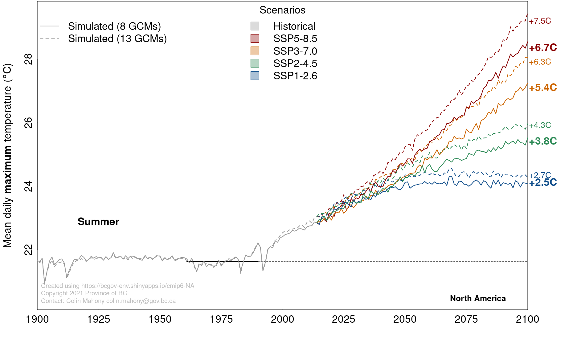
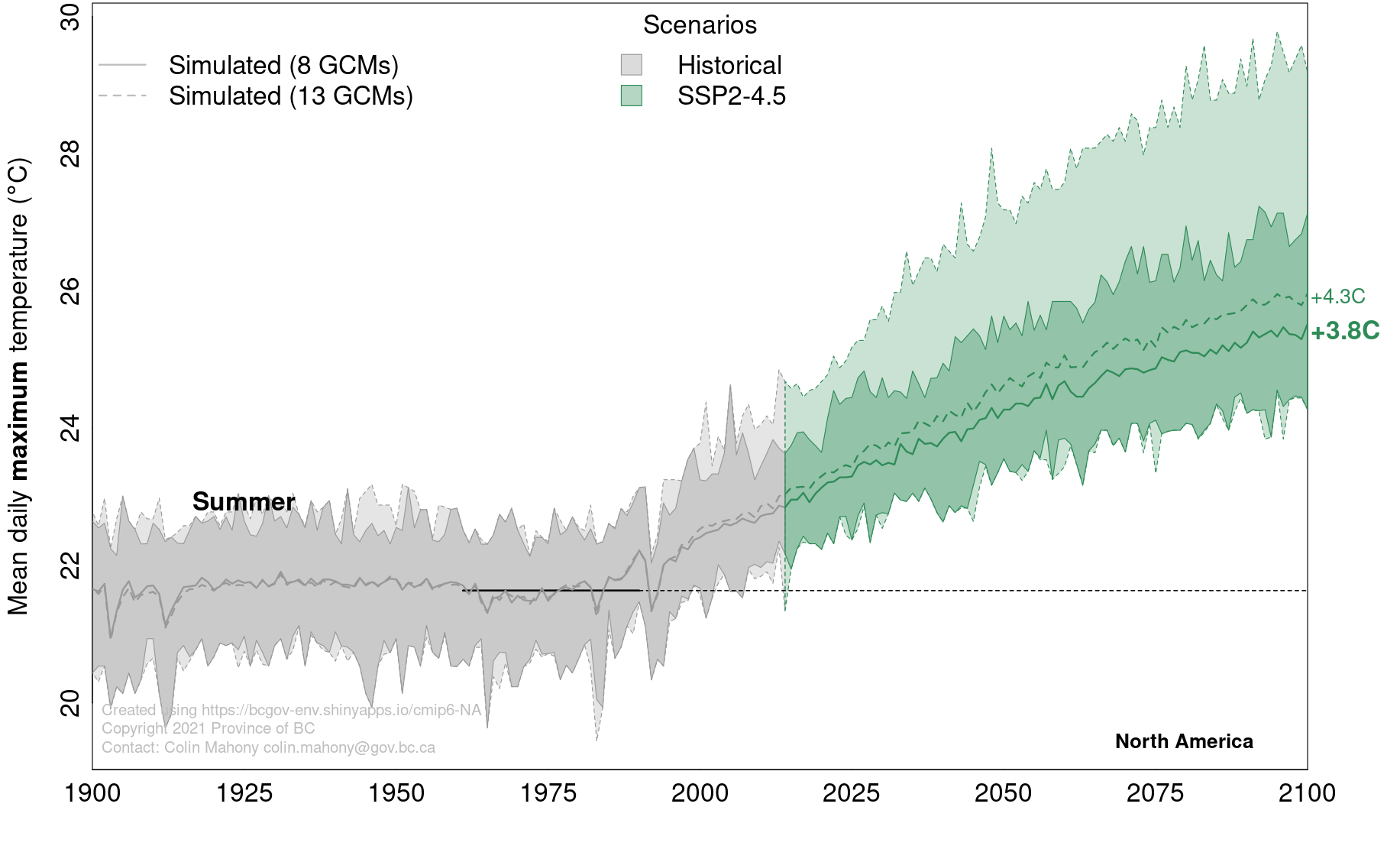 Figure 1: Comparison of
the ClimateNA 13-model ensemble (dashed lines) and 8-model ensemble
(solid lines). The variable is mean summer daily
maximum temperature (tasmax/Tmax_sm) averaged over North America. The
8-model ensemble excludes models with ECS outside the IPCC-assessed
2-5oC range. (top) Ensemble mean projections for the four
main CMIP6 marker scenarios. (bottom) Ensemble mean and full range
(min/max for all simulations of all models) for the SSP2-4.5
scenario.
Figure 1: Comparison of
the ClimateNA 13-model ensemble (dashed lines) and 8-model ensemble
(solid lines). The variable is mean summer daily
maximum temperature (tasmax/Tmax_sm) averaged over North America. The
8-model ensemble excludes models with ECS outside the IPCC-assessed
2-5oC range. (top) Ensemble mean projections for the four
main CMIP6 marker scenarios. (bottom) Ensemble mean and full range
(min/max for all simulations of all models) for the SSP2-4.5
scenario.
Reconciling the equilibrium climate sensitivity of the CMIP6 ensemble with observational constraints (Excerpted from Mahony et al. 2022)
The 13-model ensemble, like the full CMIP6 ensemble, has a mean (3.7oC) and upper limit (5.6oC) of equilibrium climate sensitivity that substantially exceeds the IPCC AR6 assessed best estimate ECS of 3oC and very likely upper limit of 5oC (Arias et al. 2021). In other words, the 13-model ensemble contains models that simulate stronger global warming than is supported by multiple lines of observational evidence. Five (38%) of the 13 models are above the IPCC AR6 assessed likely upper limit on ECS of 4oC, and two (15%) of the models are above the very likely upper limit of 5oC. If the ensemble were to strictly conform to the IPCC assessed range, there would be only two models exceeding 4oC ECS and no models exceeding 5oC, following the IPCC’s probabilistic definitions of likely (one-sided p>83%) and very likely (one-sided p>95%).
The need to reconcile the CMIP ensemble ECS range with observational constraints is a new dilemma for climate change impacts and adaptation researchers. It is long been agreed that model democracy (one model, one vote) is not a strictly valid method of assessing climate change uncertainty (Knutti 2010, Leduc et al. 2016). However, prior to CMIP6 this objection was somewhat academic since the distribution of ECS in CMIP ensembles approximately matched the (wider) range of ECS supported by other lines of evidence (Schmidt 2021). For practical purposes it was reasonable for analysts to use the multimodel ensemble spread in previous CMIP generations as a proxy for scientific uncertainty on climate change. This approach is no longer valid given the incongruence between the CMIP6 ensemble range of ECS and the IPCC assessed range (Schmidt 2021). Careful model selection is now required to avoid biasing regional climate change analyses.
There are several viable approaches to constrain CMIP6 ensembles in downscaled regional analyses. Weighting the models based on observational constraints is possible for regional analyses (Ribes et al. 2021). However, in practice many analyses will require simply selecting a subset of the CMIP6 ensemble that is closer to the IPCC assessed range, as we have done with the 8-model subset. The disadvantage of this approach is that it discards valuable information from the excluded models. The CanESM5 and UKESM1 models are advanced models from respected modeling centers, with demonstrated skill in modeling many Earth system processes (Eyring et al. 2021). Expressing variables of interest relative to the amount of regional or global warming is a widely practiced technique that facilitates inclusion of high-ECS models by removing the timing of the warming as a factor in the ensemble spread (Arias et al. 2021). It is conceivable that both techniques could be used in a single study; to use the 8-model ensemble for time-relevant analyses and a larger ensemble for analyses where the warming level is more relevant. These considerations highlight that the full CMIP6 ensemble is a somewhat arbitrary collection of non-independent models, and careful ensemble selection is necessary to achieve a meaningful representation of modeling uncertainty.
References
Arias, P. A., N. Bellouin, E. Coppola, et al. 2021. Technical Summary. Pages TS1-150 in V. Masson-Delmotte, P. Zhai, A. Pirani, et al., editors. Climate Change 2021: The Physical Science Basis. Contribution of Working Group I to the Sixth Assessment Report of the Intergovernmental Panel on Climate Change. Cambridge University Press.
Eyring, V., N. P. Gillett, K. M. A. Rao, et al. 2021. Human influence on the climate system. Pages 1–202 in V. Masson-Delmotte, P. Zhai, A. Pirani, et al., editors. Climate Change 2021: The Physical Science Basis. Contribution of Working Group I to the Sixth Assessment Report of the Intergovernmental Panel on Climate Change. Cambridge University Press.
Mahony, C.R., T. Wang, A. Hamann, and A.J. Cannon. 2022. A global climate model ensemble for downscaled monthly climate normals over North America. International Journal of Climatology. 42:5871-5891. doi.org/10.1002/joc.7566
Hausfather, Z., K. Marvel, G. A. Schmidt, J. W. Nielsen-Gammon, and M. Zelinka. 2022. Climate simulations: recognize the “hot model” problem. Nature 605:26–29.
Knutti, R. 2010. The end of model democracy? Climatic Change 102:395–404. Leduc, M., R. Laprise, R. de Elia, and L. Separovic. 2016. Is Institutional Democracy a Good Proxy for Model Independence? Journal of Climate 29:8301–8316.
Ribes, A., S. Qasmi, and N. P. Gillett. 2021. Making climate projections conditional on historical observations. Science Advances 7:1–10.
Schmidt, G.A. 2021. #NotAllModels. RealClimate. Available from: https://www.realclimate.org/index.php/archives/2021/08/notallmodels/ [Accessed 4th January 2022]