Beginner `climr` workflow

Using the downscale() function

The basic use of climr is to pass a data.table of point coordinates, IDs and elevation to downscale() and select the type of climate projection or values wanted - e.g. below we ask for future projections in two periods, using two emissions scenarios and two General Circulation Models. We also specify we want 3 individual runs of each model/scenario combination, in addition to the ensemble mean (returned by default).

library(climr)

## provide a data.frame or data.table of point coordinates, IDs and elevation
my_points <- data.frame(
  lon = c(-123.4404, -123.5064, -124.2317),
  lat = c(48.52631, 48.46807, 49.21999),
  elev = c(52, 103, 357),
  id = seq_len(3)
)

## climr query for the data.frame
ds_out <- downscale(
  xyz = my_points,
  gcms = c("GFDL-ESM4", "EC-Earth3"), # specify two global climate models
  ssps = c("ssp370", "ssp245"), # specify two greenhouse gas concentration scenarios
  gcm_periods = c("2001_2020", "2041_2060"), # specify two 20-year periods
  max_run = 3, # specify 3 individual runs for each model
  ensemble_mean = FALSE, # don't return ensemble mean of individual runs
  db_option = "local", # perform downscaling locally (instead of in database)
  vars = c("PPT", "CMD", "CMI")
)
#> .
#> .
#> .

The resulting output is a data.table, printed below:

‘ds_out’ table - Output from downscale. Outputs are shown for one location (‘id’)

id	GCM	SSP	RUN	PERIOD	PPT	CMD	CMI
1	NA	NA	NA	1961_1990	939.1875	318.3206	41.45086
1	EC-Earth3	ssp245	r15i1p1f1	2001_2020	930.9058	347.4192	37.11035
1	EC-Earth3	ssp245	r15i1p1f1	2041_2060	964.1574	375.0391	35.28234
1	EC-Earth3	ssp245	r1i1p1f1	2001_2020	950.7793	316.7011	40.82642
1	EC-Earth3	ssp245	r1i1p1f1	2041_2060	1052.9310	388.9063	42.02329
1	EC-Earth3	ssp245	r4i1p1f1	2001_2020	921.4209	362.2182	34.79205
1	EC-Earth3	ssp245	r4i1p1f1	2041_2060	944.4196	390.0571	31.17417
1	EC-Earth3	ssp370	r15i1p1f1	2001_2020	931.8873	358.3112	35.62798
1	EC-Earth3	ssp370	r15i1p1f1	2041_2060	1003.8444	358.1437	38.15592
1	EC-Earth3	ssp370	r1i1p1f1	2001_2020	887.5156	338.4092	33.32164
1	EC-Earth3	ssp370	r1i1p1f1	2041_2060	926.0189	376.1525	29.52610
1	EC-Earth3	ssp370	r4i1p1f1	2001_2020	949.9003	342.5648	37.49923
1	EC-Earth3	ssp370	r4i1p1f1	2041_2060	1043.8276	341.0114	43.32436
1	GFDL-ESM4	ssp245	r1i1p1f1	2001_2020	939.8992	318.3508	40.16827
1	GFDL-ESM4	ssp245	r1i1p1f1	2041_2060	977.5459	377.2941	35.35334
1	GFDL-ESM4	ssp245	r2i1p1f1	2001_2020	923.5054	349.3078	36.74840
1	GFDL-ESM4	ssp245	r2i1p1f1	2041_2060	1003.5399	383.7482	38.87800
1	GFDL-ESM4	ssp245	r3i1p1f1	2001_2020	944.9775	345.9026	38.66984
1	GFDL-ESM4	ssp245	r3i1p1f1	2041_2060	988.8887	383.6453	36.43479
1	GFDL-ESM4	ssp370	r1i1p1f1	2001_2020	933.8684	331.5469	39.06149
1	GFDL-ESM4	ssp370	r1i1p1f1	2041_2060	974.3047	361.3603	37.31249

Listing available options

The list_* functions (see ?list_gcm) are useful to see available options, for example:

list_gcms()
#>  [1] "ACCESS-ESM1-5" "BCC-CSM2-MR"   "CanESM5"       "CNRM-ESM2-1"  
#>  [5] "EC-Earth3"     "GFDL-ESM4"     "GISS-E2-1-G"   "INM-CM5-0"    
#>  [9] "IPSL-CM6A-LR"  "MIROC6"        "MPI-ESM1-2-HR" "MRI-ESM2-0"   
#> [13] "UKESM1-0-LL"
list_gcm_periods()
#> [1] "2001_2020" "2021_2040" "2041_2060" "2061_2080" "2081_2100"
list_ssps()
#> [1] "ssp126" "ssp245" "ssp370" "ssp585"

These functions can be used as arguments in downscale(). For example, vars = list_variables() could be specified to obtain data for all available variables, or gcms = list_gcm()[c(1,4,5,6,7,10,11,12)] could be used to specify the eight-gcm ensemble recommended by Mahony et al. (2022).

Working with raster data

A common use of climr is to obtain climate data for a user-provided raster grid. Here is some sample code showing how to do so. climr now supports native raster downscaling, so we can simply pass in a 1-layer SpatRaster containing elevation values, and climr will return a raster stack with the same extent and resolution as the input, where each layer corresponds to a variable.

library(terra)
library(data.table)

## get the sample digital elevation model (dem) provided with `climr`
dem_vancouver <- get(data("dem_vancouver")) |> 
  unwrap()

## A simple climr query. This will return the observed 1961-1990 and 2001-2020 mean annual temperature (MAT).
ds_out <- downscale(
  xyz = dem_vancouver, 
  obs_periods = "2001_2020", 
  gcms = list_gcms()[4],
  ssps = list_ssps()[2],
  gcm_periods = "2041_2060",
  vars = c("MAT")
)
#> .
#> .

plot(ds_out, range = c(2,14))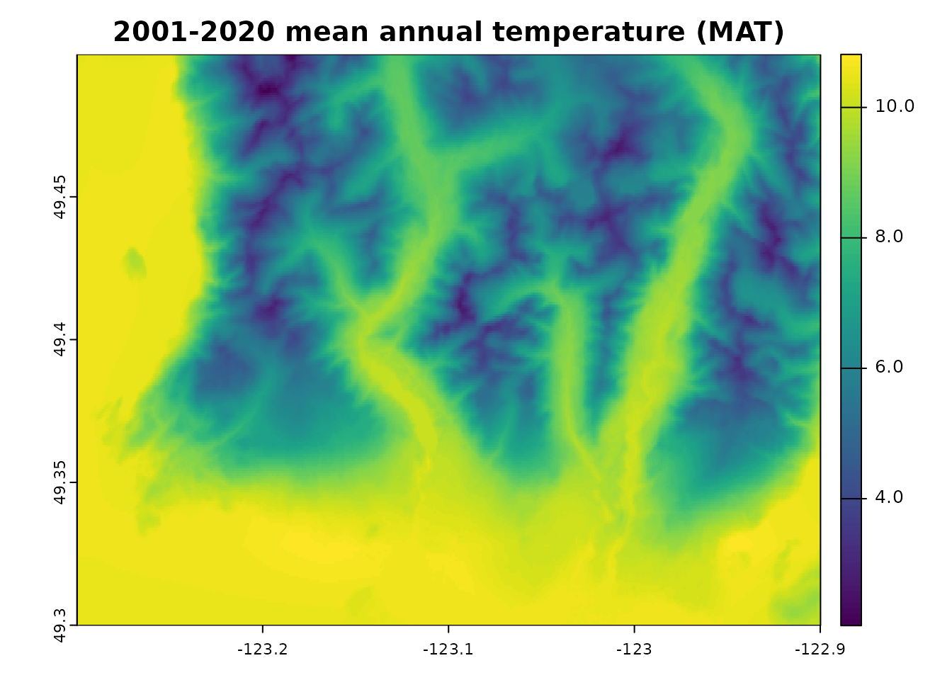

Looking under the hood

You can download and investigate the raw data that climr uses for downscaling, such as the reference climatological maps, the observational time series, and the GCM anomalies. See the section “Workflow with *_input functions and downscale” in vignette("vignettes/climr_workflow_int.Rmd") for an example.