`climr` downscaling methods
methods_downscaling.RmdDownscaling is the process of converting low-spatial-resolution
climate data to high resolution. climr adapts a downscaling
approach originally implemented in ClimateNA (Wang et al. 2016) by Dr. Tongli Wang
(University of British Columbia), Dr. Andreas Hamann (University of
Alberta), and Dave Spittlehouse (BC Ministry of Forests). This approach
downscales climate data in three stages:
- Change-factor downscaling of coarse-resolution (50-200km grid) monthly temperature and precipitation data from climate models or observational sources to high-resolution (1-4km grid);
- Elevation adjustment of temperature variables to provide scales finer than the high-resolution reference grid; and
- Calculating derived variables from the downscaled monthly temperature and precipitation variables.
Stage 1: change-factor (aka “delta”) downscaling
climr uses a simple method called change-factor
downscaling. This method is sometimes referred to as the climate imprint
method (Hunter and
Meentemeyer 2005), the delta method (Wang et al. 2016),
or simple mean bias correction (Maraun 2016). This method adds
low-spatial-resolution anomalies (e.g., from a climate model) to a
high-resolution gridded climate map (Tabor and Williams 2010). While
change-factor downscaling is too simplistic for downscaling of daily
time series or extremes indices, it is sufficient for downscaling
temperature and precipitation data at low temporal resolution (e.g.,
20-year climate averages).
The default high-resolution climate maps used by climr
are 800m gridded maps of mean daily maximum temperature
(Tmax), mean daily minimum temperature (Tmin), and
precipitation (PPT) for the 1961-1990 period. climr uses a
custom composite of climate maps from multiple sources: PRISM Climate Group (USA), Pacific
Climate Impacts Consortium (BC), and Daymet (Mexico and Canada outside
BC). There is one map for each month of the year, for a total of 36
climate maps. Here is what the July Tmax reference map looks
like in the vicinity of Vancouver, BC.
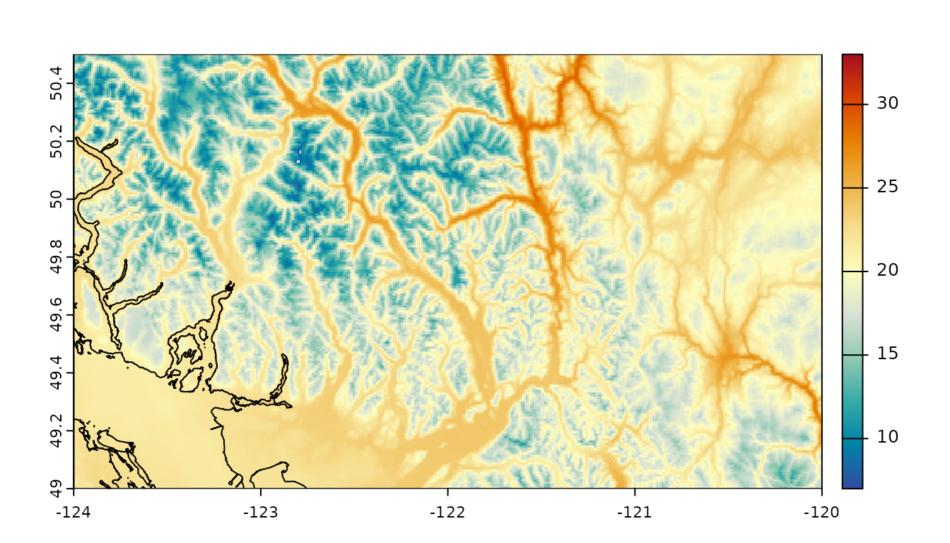
climr 1961-1990 reference climate map for July
Tmax
Global climate model data are at much lower resolution (60-200km grid scale). Here is the change in July Tmax for the EC-Earth3 global climate model for the 2041-2060 time period, relative to the model’s 1961-1990 climate. In this case, the warming is greater in areas further (eastward) from the coast.

Low-resolution anomalies (change) in July Tmax for the EC-Earth3 global climate model for the 2041-2060 time period, relative to the model’s 1961-1990 climate
To downscale the GCM projection, we first interpolate the low-resolution GCM anomaly (in this case, the temperature change from 1961-1990 to 2041-2060) to the resolution of the detailed reference climate map:
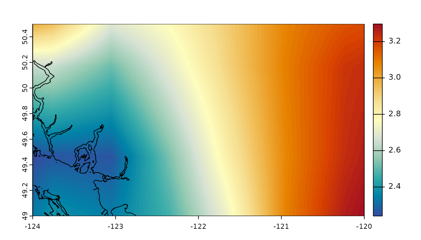
Interpolation of the low-resolution climate model anomalies to the same high resolution as the reference climate map.
Then we add these smoothed anomalies to the high-resolution 1961-1990 climate map, resulting in a high-resolution map of the simulated climate in 2041-2060.
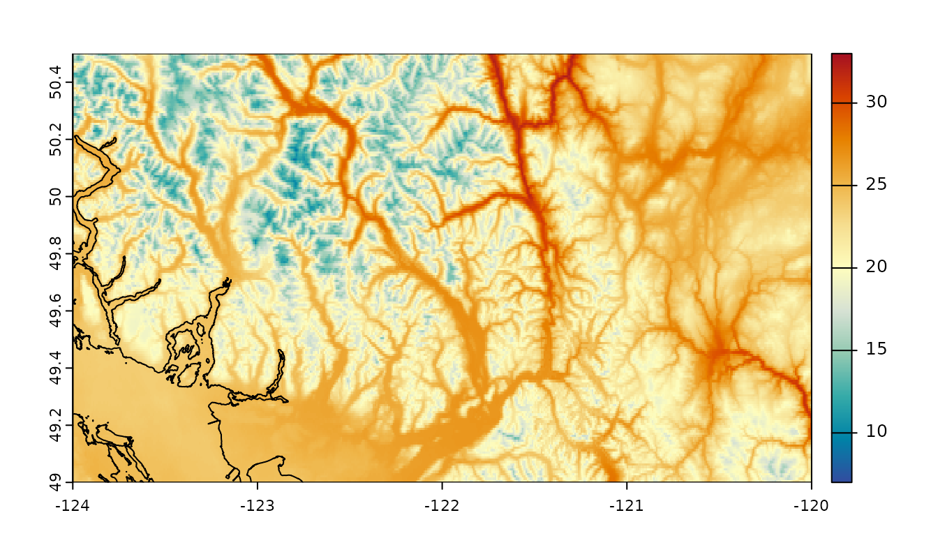
Downscaled 2041-2060 July Tmax for the EC-Earth model, resulting from addition of the interpolated low-resolution model anomalies (change factors) to the high resolution 1961-1990 reference climate.
In the case of precipitation, we multiply the reference climate by the relative anomaly (e.g., multiply by 1.07 for a 7% increase in precipitation), rather than adding the absolute anomaly.
The example above illustrates how change-factor downscaling is able to represent the effect of the ocean in reducing warming rates in coastal areas, because this large-scale effect is represented at the coarse resolution of in the global climate model. However, the downscaling here produced a uniform warming rate from valley bottom to mountain top. In reality, we would expect some large elevation-dependent differences in warming rate due for example to changes in snowpack. The inability to represent changes that occur at spatial scales smaller than the (very large) global climate model grid cells is an important weakness of change-factor downscaling and other statistical downscaling methods. Similarly, change-factor downscaling can’t represent the role of other fine-scale features like lakes, vegetation, cold-air pooling, and soil moisture. These are important considerations when interpreting the results of statistical downscaling.
Stage 2: Elevation adjustment
climr uses elevation adjustment to downscale temperature
variables to scales finer than the resolution of the reference climate
map. It does this by inferring a relationship between temperature and
elevation, known as a lapse rate, from the reference climate maps. The
local lapse rate is calculated for each grid cell of the reference
climate map using a linear regression of temperature to elevation among
the focal cell and its 8 neighbours. The gridded lapse rates are
included in the SpatRaster returned by the
input_refmap() function used above. This is the
climr lapse rate layer for July Tmax:
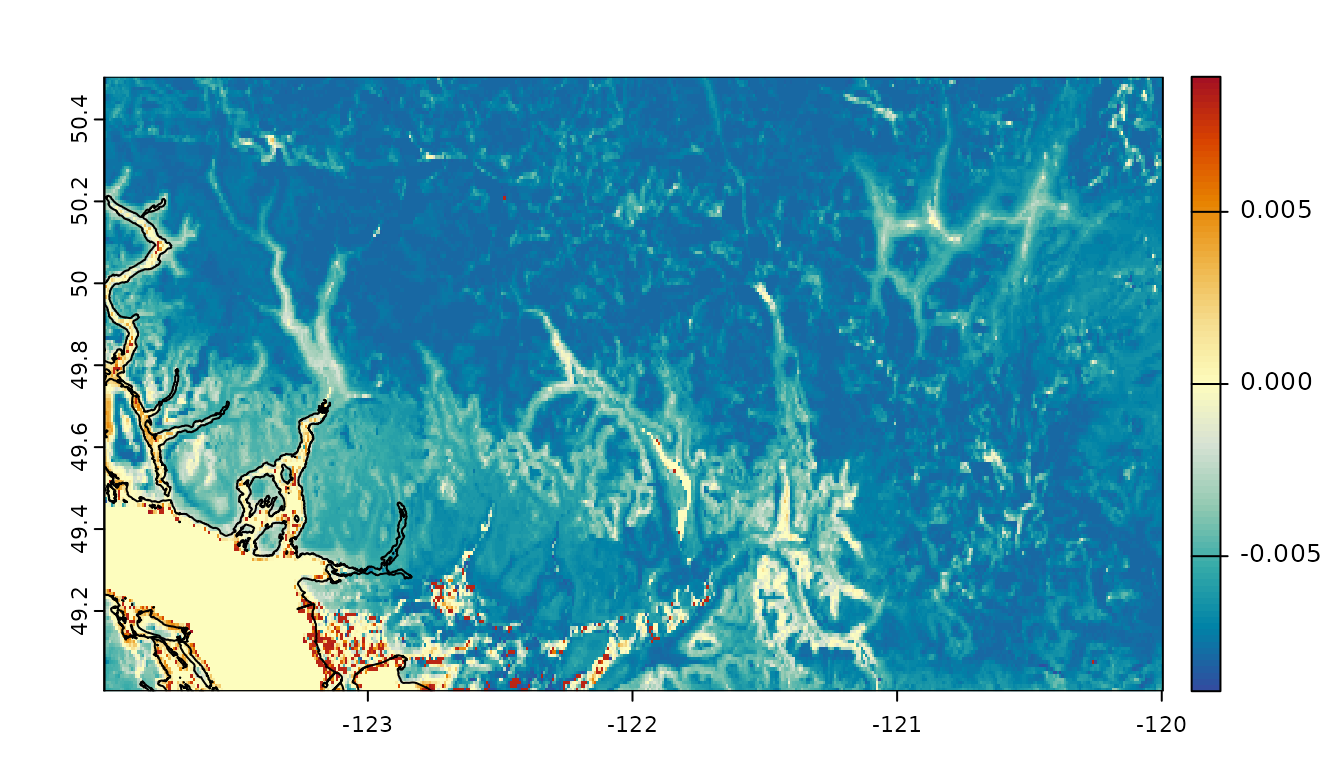
July Tmax lapse rates (change in temperature relative to elevation; oC/m) used for elevation adjustment
This example indicates that the BC PRISM maps for July
Tmax have lower lapse rates in maritime influenced mountains
(4oC/km) than in mountains with less maritime influence
(8oC/km). The map of lapse rates has artefacts in areas with
no relief; these artefacts have no consequence unless users supply
elevations for these areas that deviate substantially from realistic
ground elevations in areas of flat topography (e.g., asking
climr to provide climate values for 200m elevation on the
Fraser River delta, which is uniformly at sea level).
We can use the downscale() function with a 90m digital
elevation model (DEM) to illustrate the elevation adjustment on
Vancouver’s north shore mountains, shown below.
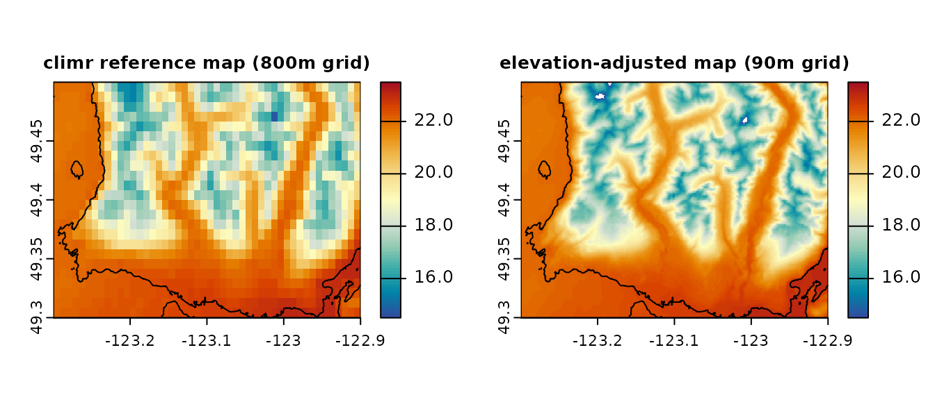
1961-1990 July Tmax in the 800m reference clmate map (left) and elevation-adjusted to a 90m grid (right).
Elevation adjustment provides a visually appealing map and can be
useful in improving precision in climate values for points of interest
in areas of steep topography. However, it is important to remember that
the climr output only represents the effects of regional
climate and elevation. Microclimatic factors such as aspect, vegetation,
water bodies, frost pooling, and soil moisture are not represented in
these maps.
By default, climr doesn’t apply elevation adjustment to
precipitation, because in most cases elevation does not influence
precipitation at scales less than 1km. Instead, precipitation at scales
finer than 800m is simply interpolated from the nearest four grid points
in the reference map. Users can choose to apply elevation-adjustment to
precipitation by selecting ppt_lr = TRUE in the
downscale() function.
Stage 3: Derived variables
The value of delta downscaling isn’t just in obtaining the new absolute values of temperature and precipitation. It allows us to calculate anomalies in other indices that don’t scale linearly with temperature or precipitation, such as degree-days or precipitation as snow.
climr currently uses the ClimateNA derived variable
equations (Wang et al.
2016). These equations are developed by fitting non-linear
models of the relationship between the variable of interest calculated
from daily weather station data and monthly temperature and/or
precipitation at these weather stations. For example, the equations for
January degree-days below 0oC and 18oC are derived
by fitting a piecewise function of these variables to January mean
temperature for the 1961-1990 period at 4891 stations across North
America, shown below in Figure 4 from Wang et al.
(2016):
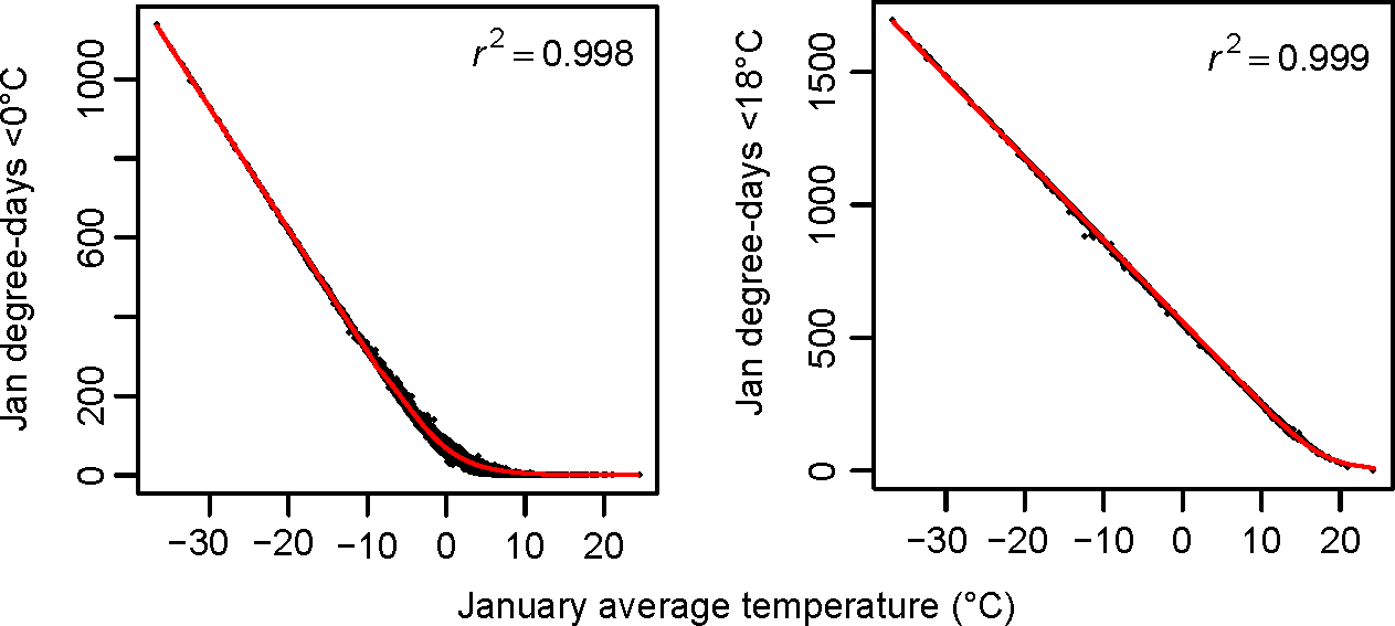
Figure 4 from Wang et al. (2016), illustrating the derivation of equations for January degree-days below 0oC and 18oC based on January mean temperature at North American weather stations
Using the climr output for the EC-Earth3 climate model,
we can compare the change in January mean temperature to change in
January degree days below 0oC in the 2041-2060 period
relative to the 1961-1990 baseline. January mean temperature is
interpolated directly from the GCM, so the only variation in the climate
change trend in this variable is the transition from one GCM grid cell
to its neighbours. In contrast, January degree-days below
0oC, while derived directly from January mean temperature,
has strong elevation-dependence in its climate change trend.
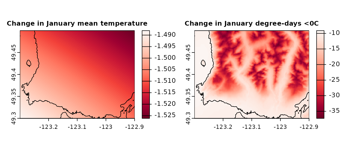
Downscaled change in January mean temperature (left) and its derived variable January degree days below 0oC (right), using the EC-Earth model simulation for 2041-2060.
climr data sources
High-resolution climate maps used by climr
The default climate maps for climr are a composite for
North America (2.4km grid scale). We compiled this composite from PRISM Climate Group (USA), Pacific
Climate Impacts Consortium (BC), and Daymet (Canada outside BC). We
recommend this reference climate map for the following reasons: (1) the
800m resolution preserves localized lapse rates (e.g. temperature
inversions) that are averaged out by the 4km ClimateNA composite; (2)
the PRISM climatology for BC is preserved by blending outwards from the
BC border; (3) lapse rates in the Alberta Rockies are better defined;
and (4) Tmin for Washington, Idaho, and Montana are
reconstructed to correct for unrealistic lapse rates.
climr provides two other options for the high-resolution
reference climate map:
- The ClimateNA composite for North America, at 4km grid scale (Wang et al. 2016). This composite is compiled from separate PRISM climate surfaces for BC, Alaska, Yukon/Alberta/Saskatchewan/Manitoba, and the contiguous US, and WorldClim (Fick and Hijmans 2017) in the remainder of the continent.
- User-supplied climate maps. the
downscale()function can accept any climate map as the reference normals. This allows the user to provide their own reference climate maps, such as: (1) Alternative publicly available gridded climatologies such as CHELSA, Daymet, or Worldclim; (2) output of weather models (e.g., WRF); or (3) custom super-high resolution climate maps for small study areas.
Historical observational time series and climates
climr provides historical observed climates for annual
time series from 1901-present and for 10-year, 20-year, and 30-year
periods from 1951-2020. These are downscaled in the same way as global
climate model data: by adding low-resolution anomalies (change factors)
to the high-resolution reference climate map. Temperature anomalies are
from the Climatic Research Unit (CRU) Time Series dataset. Precipitation
anomalies are from the Global Precipitation Climatology Centre global
dataset, which has a better representation of Canadian precipitation
stations than the CRU Time Series dataset.