Working with rasters and other spatial objects
climr_with_rasters.RmdSpatial inputs and downscale()
We often start with a spatial object of a study area (in raster or vector format) or point locations for which we want to obtain downscaled climate variables.
Bellow we show how to work with these spatial objects and
downscale().
Raster inputs
Often we have a raster of interest of the study area for which we want full coverage of downscaled climate variables.
Since downscale() accepts a table of point locations, we
need to convert the raster to a table of cell coordinates, with
elevation (‘elev’) information and unique point IDs.
Raster with elevation values (a DEM)
If the raster is a DEM, the points SpatVector inherits
the elevation cell values.
The DEM we use below has 0 elevation values in ocean areas. Since
climr is meant to be used to downscale climate variables in
land, we will “clip” (set values outside the polygon to NAs) the raster
using a land-only polygon.
library(climr)
library(terra)
library(data.table)

dem_vancouver <- get(data("dem_vancouver")) |>
  unwrap()

vancouver_poly <- get(data("vancouver_poly")) |>
  unwrap()

dem_vancouver <- mask(dem_vancouver, vancouver_poly)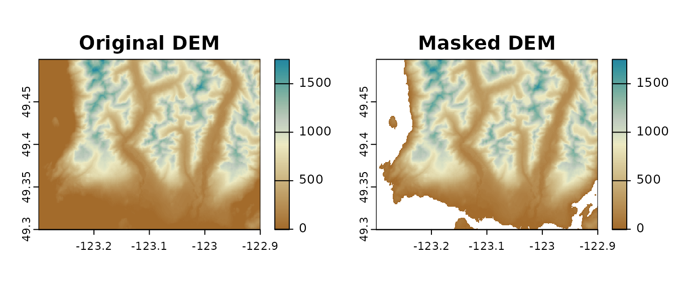
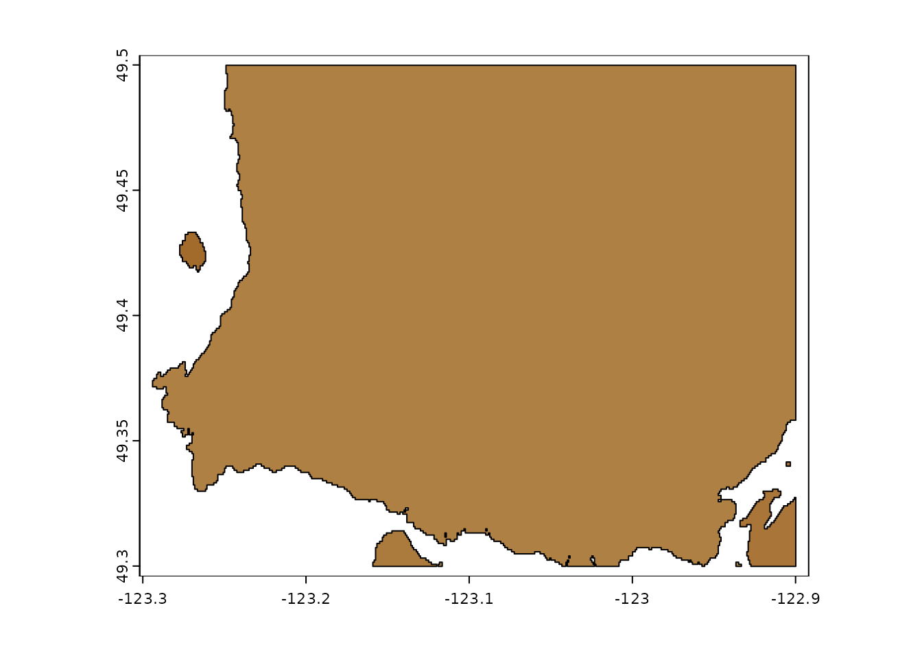
Digital Elevation Model of North Vancouver w/ and w/o values outside polygon area
When making a table of raster cell (centroid) coordinates we must
preserve the cell IDs (with
as.data.frame(..., cell = TRUE)) so that we can later
convert clirm_downscale() outputs back into raster
format.
## xy = TRUE ensures we get cell (centroid) coordinates
## cell = TRUE ensures we get cell ID numbers, which will be the point location IDs.
xyzDT <- dem_vancouver |>
  as.data.frame(., xy = TRUE, cell = TRUE) |>
  as.data.table()

## rename colums to climr standard
setnames(xyzDT, c("id", "lon", "lat", "elev"))
Note that cells with NA’s were automagically excluded.
xyzDT
#>            id       lon      lat      elev
#>         <num>     <num>    <num>     <num>
#>     1:     62 -123.2486 49.49944  16.22222
#>     2:     63 -123.2478 49.49944  39.88889
#>     3:     64 -123.2469 49.49944  81.22222
#>     4:     65 -123.2461 49.49944 139.11111
#>     5:     66 -123.2453 49.49944 179.77777
#>    ---
#> 94025: 115196 -122.9036 49.30028 112.44444
#> 94026: 115197 -122.9028 49.30028 116.44444
#> 94027: 115198 -122.9019 49.30028 128.00000
#> 94028: 115199 -122.9011 49.30028 133.33333
#> 94029: 115200 -122.9003 49.30028 136.88889
We can now pass our table of cell locations to
downscale():
## in this case there's really no need for a spatial output format
dwscl_out <- downscale(xyzDT,
  which_refmap = "auto",
  gcms = list_gcms()[1],
  ssps = list_ssps()[1],
  gcm_periods = list_gcm_periods(),
  max_run = 0L, return_refperiod = FALSE,
  vars = "MAT", out_spatial = FALSE
)
To convert the outputs back into raster format, we simply need to use the original raster use to extract the point locations as a template to make rasters of downscaled climate values.
Since the location ids match raster cell IDs, the
dwscl_out$id column is used to index raster cells climate
values when assigning downscaled MAT values.
tempRas <- rast(dem_vancouver)

dwscl_Ras <- sapply(split(dwscl_out, by = c("GCM", "PERIOD")), function(DT, tempRas) {
  tempRas[DT$id] <- DT$MAT
  return(tempRas)
}, tempRas = tempRas)

## make a stack
dwscl_Ras <- rast(dwscl_Ras)

dwscl_Ras
#> class       : SpatRaster
#> dimensions  : 240, 480, 5  (nrow, ncol, nlyr)
#> resolution  : 0.0008333333, 0.0008333333  (x, y)
#> extent      : -123.2999, -122.8999, 49.29986, 49.49986  (xmin, xmax, ymin, ymax)
#> coord. ref. : lon/lat WGS 84 (EPSG:4326)
#> source(s)   : memory
#> names       : ACCESS~1_2020, ACCESS~1_2040, ACCESS~1_2060, ACCESS~1_2080, ACCESS~1_2100
#> min values  :      3.011241,      4.083216,      4.864598,      5.315447,      5.305784
#> max values  :     11.770973,     12.841200,     13.613663,     14.062831,     14.053918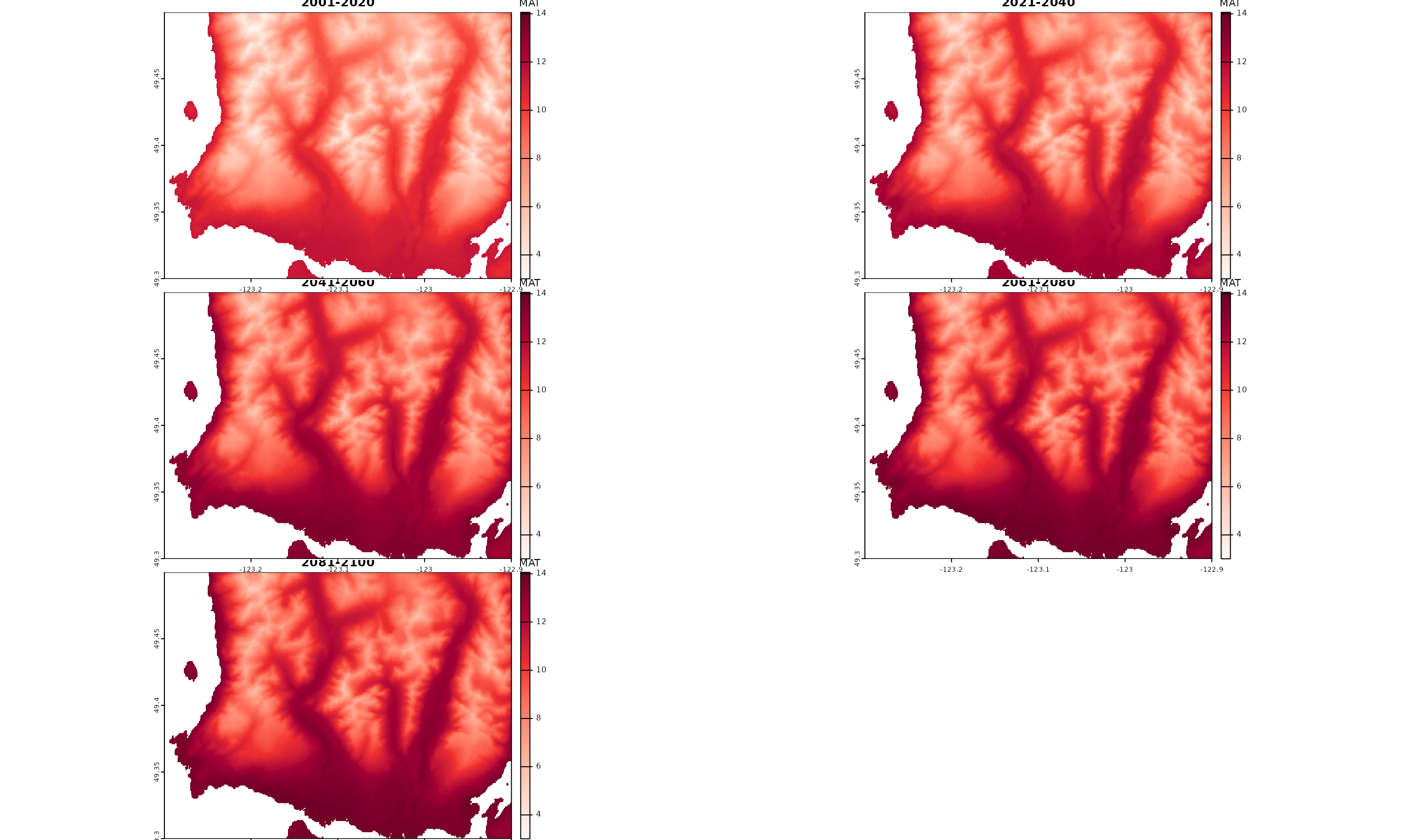
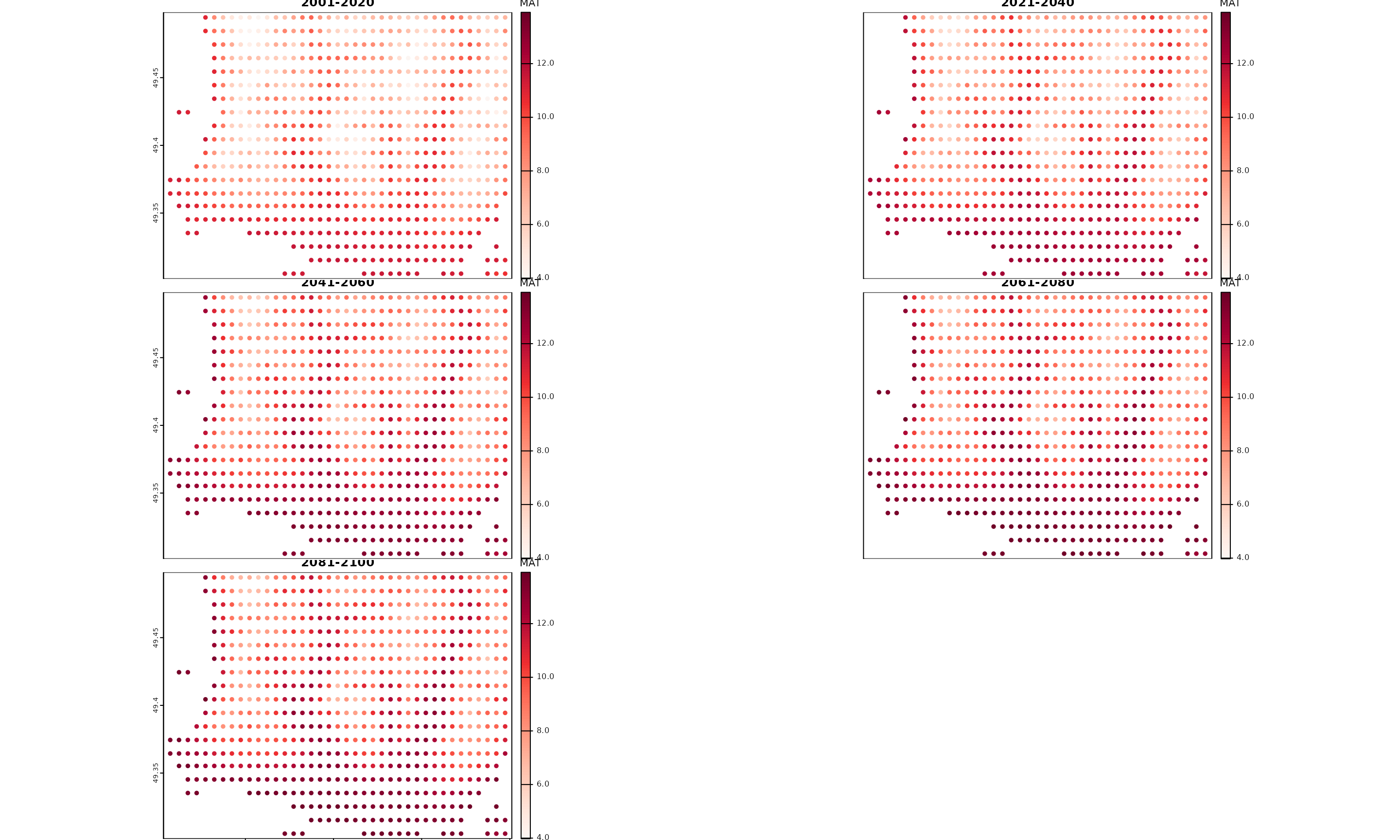
downscale() outputs converted to raster layers
Raster without elevation values
If the raster is not a DEM, we need to obtain elevation for each of the points extracted from the raster cells. This can be done by extracting elevation values from a DEM raster at the first raster’s cell centroid coordinates.
The DEM’s resolution doesn’t need to match the first raster’s resolution.
Here we start with a raster of biogeoclimatc zones for North Vancouver and use a lower resolution DEM to obtain elevation values.
Again, we clip it to land areas.
## get point locations from raster of interest
BECz_vancouver_ras <- get(data("BECz_vancouver_ras")) |>
  unwrap()

BECz_vancouver_ras <- mask(BECz_vancouver_ras, vancouver_poly)

## raster to data.table and rename columns to climr standard
xyzDT <- BECz_vancouver_ras |>
  as.data.frame(., xy = TRUE, cell = TRUE) |>
  as.data.table()
setnames(xyzDT, c("id", "lon", "lat", "ZONE"))

## now extract elevation values at each cell centroid coordinate
## from a DEM raster
dem_vancouver_lowres <- get(data(dem_vancouver_lowres)) |>
  unwrap()

xyzDT$elev <- extract(dem_vancouver_lowres, xyzDT[, .(lon, lat)])[names(dem_vancouver_lowres)]
par(mfrow = c(1, 2))
plot(BECz_vancouver_ras, main = "BGC zones N Vancouver")
plot(dem_vancouver_lowres,
  main = "Low res. DEM",
  col = hcl.colors(100, "Earth")
)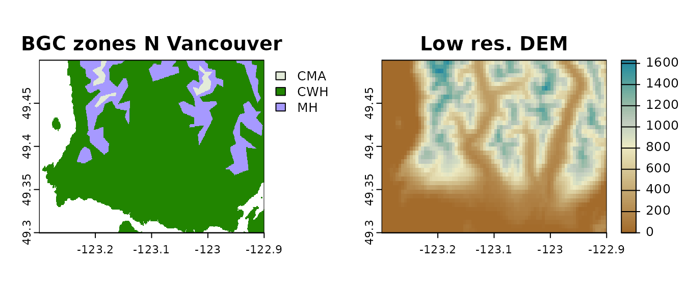
Rasters used to derive point locations (left) and elevation values (right).
The process to convert the downscaled data to raster format is the
same as before, because we again used the raster cell IDs as point
location IDs (xyzDT$id):
dwscl_out <- downscale(xyzDT,
  which_refmap = "auto",
  gcms = list_gcms()[1],
  ssps = list_ssps()[1],
  gcm_periods = list_gcm_periods(),
  max_run = 0L, return_refperiod = FALSE,
  vars = "MAT", out_spatial = FALSE
)

tempRas <- rast(BECz_vancouver_ras)

dwscl_Ras <- sapply(split(dwscl_out, by = c("GCM", "PERIOD")), function(DT, tempRas) {
  tempRas[DT$id] <- DT$MAT
  return(tempRas)
}, tempRas = tempRas)

## make a stack
dwscl_Ras <- rast(dwscl_Ras)
Lowering an input raster resolution
We may want to downscale climate at a coarser resolution than the, e.g., DEM raster layer we have at hand:
vancouver_poly <- get(data("vancouver_poly")) |>
  unwrap()
dem_vancouver <- get(data("dem_vancouver")) |>
  unwrap()

dem_vancouver <- mask(dem_vancouver, vancouver_poly)

## extract points at a coarser scale, but elevation at original scale
lowRes_ras <- rast(dem_vancouver)
lowRes_ras <- project(lowRes_ras, crs(lowRes_ras), res = 0.01)

lowRes_ras[] <- 1
lowRes_ras <- mask(lowRes_ras, vancouver_poly) ## set water back to NA

lowRes_points <- as.points(lowRes_ras)
lowRes_points$id <- 1:nrow(lowRes_points)

xyzDT <- extract(dem_vancouver, lowRes_points, xy = TRUE) |>
  as.data.table()
setnames(xyzDT, c("id", "elev", "lon", "lat"))

## exclude NAs
xyzDT <- xyzDT[complete.cases(xyzDT)]
lowRes_points <- lowRes_points[lowRes_points$id %in% xyzDT$id, ]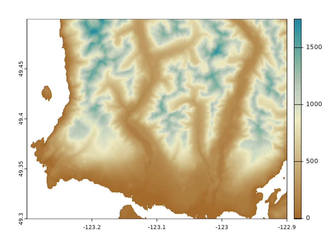
Points extracted from raster
As before, pass your data.table of point locations to
downscale:
dwscl_out <- downscale(xyzDT,
  which_refmap = "auto",
  gcms = list_gcms()[1],
  ssps = list_ssps()[1],
  gcm_periods = list_gcm_periods(),
  max_run = 0L, return_refperiod = FALSE,
  vars = "MAT", out_spatial = TRUE
)
Plot of spatial outputs from downscale() using more spaced
point locations
Vector inputs/outputs
Point vector data
The process is again similar to the above.
If the points have elevation information we simply need to convert
them to a data.table. In this case, point IDs need to be
added to the data.table afterwards.
If they don’t have elevation information, then we need to obtain it. In the example below we start with a set of points in North Vancouver, BC, Canada, for which we get elevation values from a Digital Elevation Model (DEM) raster.
The terra::extract() function outputs a
data.frame with point IDs, the extracted values and,
optionally x/y coordinates. So we need simply to use this output to
create our xyzDT table for downscale().
To get point-type outputs simply set
downscale(..., out_spatial = TRUE).
vancouver_points <- get(data("vancouver_points")) |>
  unwrap()
dem_vancouver <- get(data("dem_vancouver")) |>
  unwrap()

xyzDT <- extract(dem_vancouver, vancouver_points, xy = TRUE) |>
  as.data.table()
setnames(xyzDT, c("id", "elev", "lon", "lat"))

dwscl_out <- downscale(xyzDT,
  which_refmap = "auto",
  gcms = list_gcms()[1],
  ssp = list_ssps()[1],
  gcm_periods = list_gcm_periods(),
  vars = "MAT", max_run = 0L,
  return_refperiod = FALSE,
  out_spatial = TRUE
)
dwscl_out
#> class : SpatVector
#> geometry : points
#> dimensions : 5000, 7 (geometries, attributes)
#> extent : -123.2828, -122.9003, 49.30028, 49.49944 (xmin, xmax, ymin, ymax)
#> coord. ref. : +proj=longlat +datum=WGS84 +no_defs
#> names : elev id GCM SSP RUN PERIOD MAT
#> type : <num> <num> <chr> <chr> <chr> <chr> <num>
#> values : 233.1 1 ACCESS-ESM1-5 ssp126 ensembleMean 2001_2020 10.32
#> 233.1 1 ACCESS-ESM1-5 ssp126 ensembleMean 2021_2040 11.39
#> 233.1 1 ACCESS-ESM1-5 ssp126 ensembleMean 2041_2060 12.16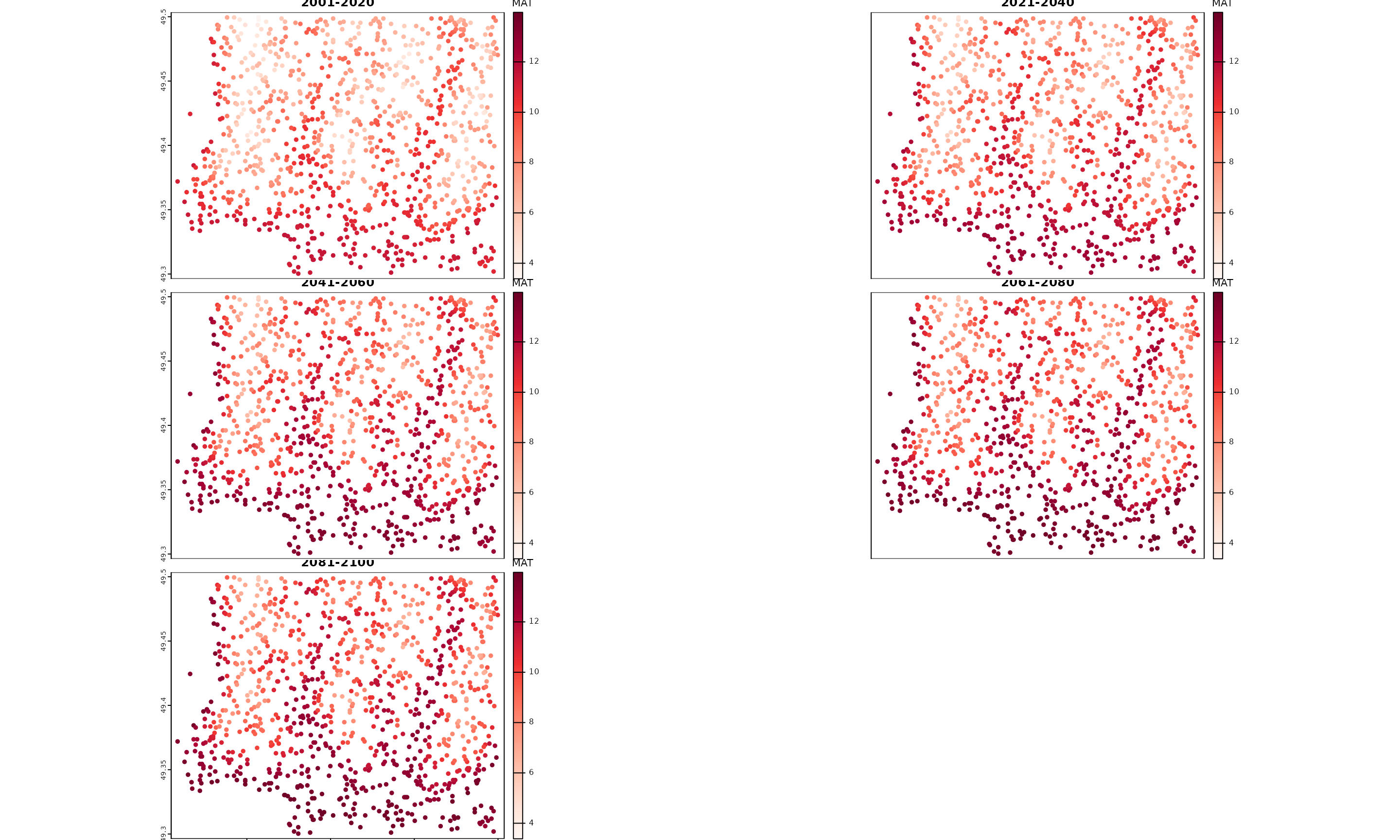
Plot of spatial outputs from downscale()
Polygon vector data
We assume here that your polygon data refers to an area (or several) for which you want downscaled climate variables for.
Because each polygon is associated with a single value per attribute
or field, the polygons will need to be sampled/combined with the points
where downscaling will happen. In the examples above we showed how to
use a polygon to mask a raster or points dataset before creating the
xyzDT table, which would be a way to achieve this.
Here, we show another example of how points derived from the polygon centroids.
using polygon centroids
We advise against doing this unless your polygons are so small that the centroid reflects the overall polygon’s climate conditions.
vancouver_poly <- get(data("vancouver_poly")) |>
  unwrap()
dem_vancouver <- get(data("dem_vancouver")) |>
  unwrap()

centrds <- centroids(vancouver_poly, inside = TRUE)

## get polygon areas and exclude very large polygon centroids
centrds$area <- expanse(vancouver_poly)
centrds <- centrds[centrds$area < 50000, ]

## we retained only 3 points

xyzDT <- extract(dem_vancouver, centrds, xy = TRUE) |>
  as.data.table()
setnames(xyzDT, c("id", "elev", "lon", "lat"))

dwscl_outGrid <- downscale(xyzDT,
  which_refmap = "auto",
  gcms = list_gcms()[1],
  ssp = list_ssps()[1],
  gcm_periods = list_gcm_periods(),
  max_run = 0L, return_refperiod = FALSE,
  vars = "MAT", out_spatial = TRUE
)
Excluded (grey) and retained (blue) polygon centroids