5 Manipulating Data Frames with dplyr
At this point, you’ve seen it all: in the last lesson, we toured all the basic data types and data structures in R. Everything you do will be a manipulation of those tools. But most of the time, the star of the show is the data frame—the table that we created by loading information from a csv file. In this lesson, we’ll learn a few more things about working with data frames including how you might summarize a dataframe by a grouping variable, including only certain observations in your summary. We will do this with the popular package dplyr.
Rows: 3 Columns: 3
── Column specification ────────────────────────────────────────────────────────
Delimiter: ","
chr (1): coat
dbl (2): weight, likes_string

ℹ Use `spec()` to retrieve the full column specification for this data.
ℹ Specify the column types or set `show_col_types = FALSE` to quiet this message.
We can find the size and various other attributes of our data with a few handy functions:
nrow(cats)[1] 3
ncol(cats)[1] 3
dim(cats)[1] 3 3
names(cats)[1] "coat" "weight" "likes_string"
str(cats)spc_tbl_ [3 × 3] (S3: spec_tbl_df/tbl_df/tbl/data.frame)
$ coat : chr [1:3] "calico" "black" "tabby"
$ weight : num [1:3] 2.1 5 3.2
$ likes_string: num [1:3] 1 0 1
- attr(*, "spec")=
.. cols(
.. coat = col_character(),
.. weight = col_double(),
.. likes_string = col_double()
.. )
- attr(*, "problems")=<externalptr> A way to get a nice overall view of a data frame is to use the summary function. This function can be used on various objects in R. For data frames, summary yields a numeric, tabular, or descriptive summary of each column. Factor columns are summarized by the number of items in each level, numeric or integer columns by the descriptive statistics (quartiles and mean), and character columns by its length, class, and mode.
summary(cats) coat weight likes_string
Length:3 Min. :2.100 Min. :0.0000
Class :character 1st Qu.:2.650 1st Qu.:0.5000
Mode :character Median :3.200 Median :1.0000
Mean :3.433 Mean :0.6667
3rd Qu.:4.100 3rd Qu.:1.0000
Max. :5.000 Max. :1.0000 A really nice feature of RStudio is that it allows us to view our data in a
very readable and familiar way. Go ahead and click on the name of the cats
data frame in the environment pane.
Note that this is a read-only view, it’s not editable (which is a good thing!)
5.1 Introducing the Gapminder data
So far, you have seen the basics of manipulating data frames with our cat data;
now let’s use those skills to digest a more realistic dataset. Let’s read in the
gapminder dataset that we downloaded previously and assign it to a data frame called gapminder:
gapminder <- read_csv("data/gapminder_data.csv")Rows: 1704 Columns: 6
── Column specification ────────────────────────────────────────────────────────
Delimiter: ","
chr (2): country, continent
dbl (4): year, pop, lifeExp, gdpPercap
ℹ Use `spec()` to retrieve the full column specification for this data.
ℹ Specify the column types or set `show_col_types = FALSE` to quiet this message.5.1.1 Challenge 1 (5 minutes)
How many rows and columns does
gapminderhave?What kind of data is in the
popandcontinentcolumns?Solution to challenge 1
dim(gapminder)[1] 1704 6nrow(gapminder)[1] 1704ncol(gapminder)[1] 6str(gapminder)spc_tbl_ [1,704 × 6] (S3: spec_tbl_df/tbl_df/tbl/data.frame) $ country : chr [1:1704] "Afghanistan" "Afghanistan" "Afghanistan" "Afghanistan" ... $ year : num [1:1704] 1952 1957 1962 1967 1972 ... $ pop : num [1:1704] 8425333 9240934 10267083 11537966 13079460 ... $ continent: chr [1:1704] "Asia" "Asia" "Asia" "Asia" ... $ lifeExp : num [1:1704] 28.8 30.3 32 34 36.1 ... $ gdpPercap: num [1:1704] 779 821 853 836 740 ... - attr(*, "spec")= .. cols( .. country = col_character(), .. year = col_double(), .. pop = col_double(), .. continent = col_character(), .. lifeExp = col_double(), .. gdpPercap = col_double() .. ) - attr(*, "problems")=<externalptr>summary(gapminder)country year pop continent Length:1704 Min. :1952 Min. :6.001e+04 Length:1704 Class :character 1st Qu.:1966 1st Qu.:2.794e+06 Class :character Mode :character Median :1980 Median :7.024e+06 Mode :character Mean :1980 Mean :2.960e+07 3rd Qu.:1993 3rd Qu.:1.959e+07 Max. :2007 Max. :1.319e+09 lifeExp gdpPercap Min. :23.60 Min. : 241.2 1st Qu.:48.20 1st Qu.: 1202.1 Median :60.71 Median : 3531.8 Mean :59.47 Mean : 7215.3 3rd Qu.:70.85 3rd Qu.: 9325.5 Max. :82.60 Max. :113523.1
The first thing we should always do is check out what the data looks like with
str() or summary():
str(gapminder)spc_tbl_ [1,704 × 6] (S3: spec_tbl_df/tbl_df/tbl/data.frame)
$ country : chr [1:1704] "Afghanistan" "Afghanistan" "Afghanistan" "Afghanistan" ...
$ year : num [1:1704] 1952 1957 1962 1967 1972 ...
$ pop : num [1:1704] 8425333 9240934 10267083 11537966 13079460 ...
$ continent: chr [1:1704] "Asia" "Asia" "Asia" "Asia" ...
$ lifeExp : num [1:1704] 28.8 30.3 32 34 36.1 ...
$ gdpPercap: num [1:1704] 779 821 853 836 740 ...
- attr(*, "spec")=
.. cols(
.. country = col_character(),
.. year = col_double(),
.. pop = col_double(),
.. continent = col_character(),
.. lifeExp = col_double(),
.. gdpPercap = col_double()
.. )
- attr(*, "problems")=<externalptr>
summary(gapminder$country) Length Class Mode
1704 character character Miscellaneous Tips
- Files can also be downloaded directly from the Internet into a local
folder of your choice onto your computer using the
download.filefunction. Theread_csvfunction can then be executed to read the downloaded file from the download location, for example,
download.file("https://raw.githubusercontent.com/swcarpentry/r-novice-gapminder/gh-pages/_episodes_rmd/data/gapminder_data.csv", destfile = "data/gapminder_data.csv")
gapminder <- read_csv("data/gapminder_data.csv")- Alternatively, you can also read in files directly into R from the Internet by replacing the file paths with a web address in
read_csv. One should note that in doing this no local copy of the csv file is first saved onto your computer. For example,
gapminder <- read_csv("https://raw.githubusercontent.com/swcarpentry/r-novice-gapminder/gh-pages/_episodes_rmd/data/gapminder_data.csv")- You can read directly from excel spreadsheets without converting them to plain text first by using the readxl package.
We’ll also likely want to know what the titles of all the columns are, so we can ask for them:
names(gapminder)[1] "country" "year" "pop" "continent" "lifeExp" "gdpPercap"At this stage, it’s important to ask ourselves if the structure R is reporting matches our intuition or expectations; do the basic data types reported for each column make sense? If not, we need to sort any problems out now before they turn into bad surprises down the road, using what we’ve learned about how R interprets data, and the importance of strict consistency in how we record our data.
Once we’re happy that the data types and structures seem reasonable, it’s time to start digging into our data proper. Check out the first few lines:
head(gapminder)# A tibble: 6 × 6
country year pop continent lifeExp gdpPercap
<chr> <dbl> <dbl> <chr> <dbl> <dbl>
1 Afghanistan 1952 8425333 Asia 28.8 779.
2 Afghanistan 1957 9240934 Asia 30.3 821.
3 Afghanistan 1962 10267083 Asia 32.0 853.
4 Afghanistan 1967 11537966 Asia 34.0 836.
5 Afghanistan 1972 13079460 Asia 36.1 740.
6 Afghanistan 1977 14880372 Asia 38.4 786.Another very helpful function for looking at your data is the unique()
function, to see the unique values in a particular column:
unique(gapminder$continent)[1] "Asia" "Europe" "Africa" "Americas" "Oceania" Manipulation of dataframes means many things to many researchers, we often select certain observations (rows) or variables (columns), we often group the data by a certain variable(s), or we even calculate summary statistics. We can do these types of operations using the normal base R operations:
mean(gapminder$gdpPercap)[1] 7215.327The question here is how might you summarize and split by some group you might be interested in.
5.2 The dplyr package
Luckily, the dplyr
package provides a number of very useful functions for manipulating dataframes
in a way that will reduce repetition, reduce the probability of making
errors, and probably even save you some typing. As an added bonus, you might
even find the dplyr grammar easier to read.
Here we’re going to cover 5 of the most commonly used functions as well as using
pipes (%>%) to combine them.
If you have have not installed this package earlier, please do so:
install.packages('dplyr')Now let’s load the package:
5.3 Using select()
If, for example, we wanted to move forward with only a few of the variables in
our dataframe we could use the select() function. This will keep only the
variables you select.
year_country_gdp <- select(gapminder, year, country, gdpPercap)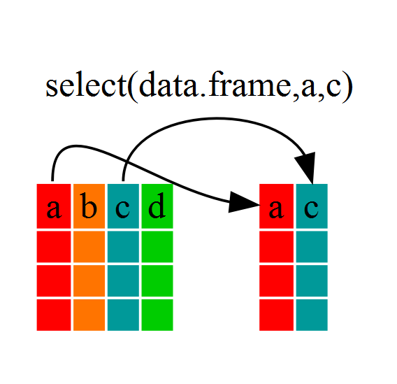
5.4 Using filter()
To select on some subset of rows:
filter(gapminder, continent == "Europe")# A tibble: 360 × 6
country year pop continent lifeExp gdpPercap
<chr> <dbl> <dbl> <chr> <dbl> <dbl>
1 Albania 1952 1282697 Europe 55.2 1601.
2 Albania 1957 1476505 Europe 59.3 1942.
3 Albania 1962 1728137 Europe 64.8 2313.
4 Albania 1967 1984060 Europe 66.2 2760.
5 Albania 1972 2263554 Europe 67.7 3313.
6 Albania 1977 2509048 Europe 68.9 3533.
7 Albania 1982 2780097 Europe 70.4 3631.
8 Albania 1987 3075321 Europe 72 3739.
9 Albania 1992 3326498 Europe 71.6 2497.
10 Albania 1997 3428038 Europe 73.0 3193.
# … with 350 more rowsOr select another subset of rows:
filter(gapminder, pop > 1000000)# A tibble: 1,524 × 6
country year pop continent lifeExp gdpPercap
<chr> <dbl> <dbl> <chr> <dbl> <dbl>
1 Afghanistan 1952 8425333 Asia 28.8 779.
2 Afghanistan 1957 9240934 Asia 30.3 821.
3 Afghanistan 1962 10267083 Asia 32.0 853.
4 Afghanistan 1967 11537966 Asia 34.0 836.
5 Afghanistan 1972 13079460 Asia 36.1 740.
6 Afghanistan 1977 14880372 Asia 38.4 786.
7 Afghanistan 1982 12881816 Asia 39.9 978.
8 Afghanistan 1987 13867957 Asia 40.8 852.
9 Afghanistan 1992 16317921 Asia 41.7 649.
10 Afghanistan 1997 22227415 Asia 41.8 635.
# … with 1,514 more rowsAbove we used ‘normal’ grammar, but the strengths of dplyr lie in combining
several functions using pipes. This
description is very useful:
I woke up %>%
  showered %>%
  dressed %>%
  had coffee %>%
  came to an R workshop
Since the pipes grammar is unlike anything we’ve seen in R before, let’s repeat what we’ve done above using pipes.
To help you understand why we wrote that in that way, let’s walk through it step
by step. First we summon the gapminder dataframe and pass it on, using the pipe
symbol %>%, to the next step, which is the select() function. In this case
we don’t specify which data object we use in the select() function since in
gets that from the previous pipe. Fun Fact: There is a good chance you have
encountered pipes before in the shell. In R, a pipe symbol is %>% while in the
shell it is | but the concept is the same!
5.5 Using filter() with pipes
If we now wanted to move forward with the above, but only with European
countries, we can combine select and filter
year_country_gdp_euro <- gapminder %>%
    filter(continent == "Europe") %>%
    select(year, country, gdpPercap)
5.5.1 Challenge 2 (10 minutes)
Write a single command (which can span multiple lines and includes pipes) that will produce a dataframe that has the African values for
lifeExp,countryandyear, but not for other Continents. How many rows does your dataframe have and why?
As with last time, first we pass the gapminder dataframe to the filter()
function, then we pass the filtered version of the gapminder dataframe to the
select() function. Note: The order of operations is very important in this
case. If we used ‘select’ first, filter would not be able to find the variable
continent since we would have removed it in the previous step.
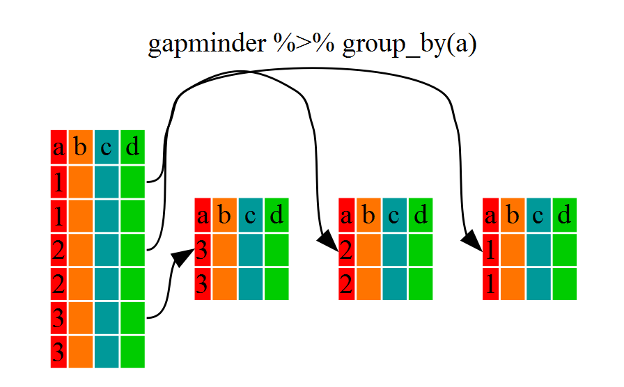
5.6 Using group_by() and summarize()
Now, we were supposed to be reducing the error prone repetitiveness of what can
be done with base R, but up to now we haven’t done that since we would have to
repeat the above for each continent. Instead of filter(), which will only pass
observations that meet your criteria (in the above: continent=="Europe"), we
can use group_by(), which will essentially use every unique criteria that you
could have used in filter.
gapminder# A tibble: 1,704 × 6
country year pop continent lifeExp gdpPercap
<chr> <dbl> <dbl> <chr> <dbl> <dbl>
1 Afghanistan 1952 8425333 Asia 28.8 779.
2 Afghanistan 1957 9240934 Asia 30.3 821.
3 Afghanistan 1962 10267083 Asia 32.0 853.
4 Afghanistan 1967 11537966 Asia 34.0 836.
5 Afghanistan 1972 13079460 Asia 36.1 740.
6 Afghanistan 1977 14880372 Asia 38.4 786.
7 Afghanistan 1982 12881816 Asia 39.9 978.
8 Afghanistan 1987 13867957 Asia 40.8 852.
9 Afghanistan 1992 16317921 Asia 41.7 649.
10 Afghanistan 1997 22227415 Asia 41.8 635.
# … with 1,694 more rows# A tibble: 1,704 × 6
# Groups: continent [5]
country year pop continent lifeExp gdpPercap
<chr> <dbl> <dbl> <chr> <dbl> <dbl>
1 Afghanistan 1952 8425333 Asia 28.8 779.
2 Afghanistan 1957 9240934 Asia 30.3 821.
3 Afghanistan 1962 10267083 Asia 32.0 853.
4 Afghanistan 1967 11537966 Asia 34.0 836.
5 Afghanistan 1972 13079460 Asia 36.1 740.
6 Afghanistan 1977 14880372 Asia 38.4 786.
7 Afghanistan 1982 12881816 Asia 39.9 978.
8 Afghanistan 1987 13867957 Asia 40.8 852.
9 Afghanistan 1992 16317921 Asia 41.7 649.
10 Afghanistan 1997 22227415 Asia 41.8 635.
# … with 1,694 more rowsYou will notice that the structure of the dataframe where we used group_by()
(grouped_df) is not the same as the original gapminder (data.frame). A
grouped_df can be thought of as a list where each item in the list is a
data.frame which contains only the rows that correspond to the a particular
value continent (at least in the example above).
5.7 Using summarize()
The above was a bit on the uneventful side but group_by() is much more
exciting in conjunction with summarize(). This will allow us to create new
variable(s) by using functions that repeat for each of the continent-specific
data frames. That is to say, using the group_by() function, we split our
original dataframe into multiple pieces, then we can run functions
(e.g. mean() or sd()) within summarize().
gdp_bycontinents <- gapminder %>%
    group_by(continent) %>%
    summarize(mean_gdpPercap = mean(gdpPercap))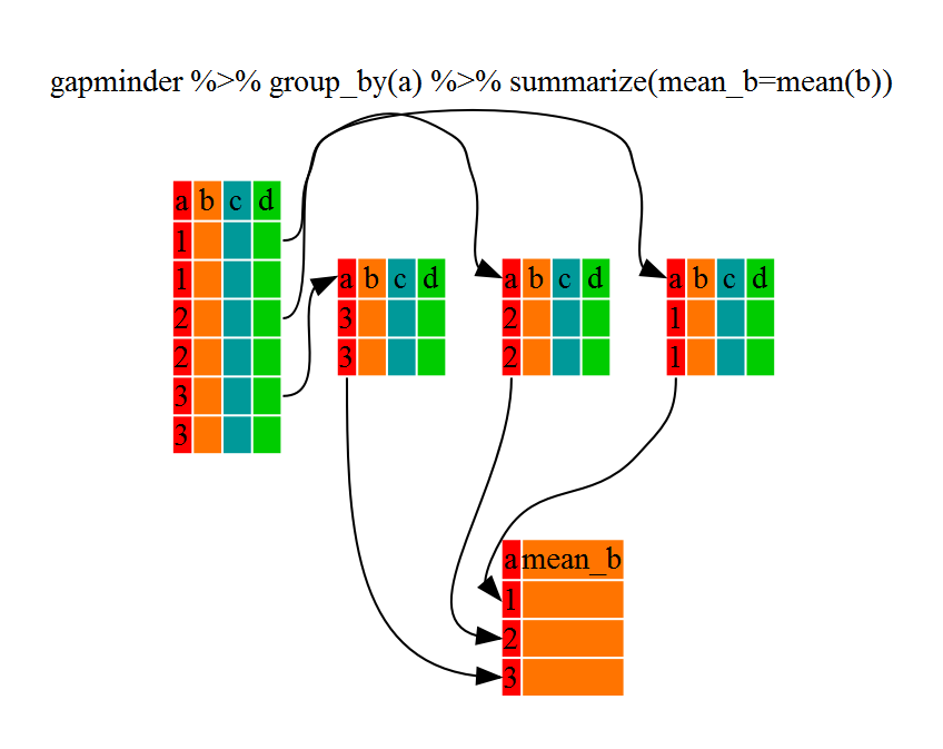
# A tibble: 5 × 2
  continent mean_gdpPercap
  <chr>              <dbl>
1 Africa             2194.
2 Americas           7136.
3 Asia               7902.
4 Europe            14469.
5 Oceania           18622.
That allowed us to calculate the mean gdpPercap for each continent, but it gets even better.
5.7.1 Challenge 3 (10 minutes)
Calculate the average life expectancy per country. Which has the longest average life expectancy and which has the shortest average life expectancy?
Solution to challenge 3
lifeExp_bycountry <- gapminder %>%
   group_by(country) %>%
   summarize(mean_lifeExp = mean(lifeExp))
lifeExp_bycountry %>%
   filter(mean_lifeExp == min(mean_lifeExp) | mean_lifeExp == max(mean_lifeExp))
# A tibble: 2 × 2 country mean_lifeExp <chr> <dbl> 1 Iceland 76.5 2 Sierra Leone 36.8Another way to do this is to use the
dplyrfunctionarrange(), which arranges the rows in a data frame according to the order of one or more variables from the data frame. It has similar syntax to other functions from thedplyrpackage. You can usedesc()insidearrange()to sort in descending order.# A tibble: 1 × 2 country mean_lifeExp <chr> <dbl> 1 Sierra Leone 36.8# A tibble: 1 × 2 country mean_lifeExp <chr> <dbl> 1 Iceland 76.5
The function group_by() allows us to group by multiple variables. Let’s group by year and continent.
gdp_bycontinents_byyear <- gapminder %>%
    group_by(continent, year) %>%
    summarize(mean_gdpPercap = mean(gdpPercap))
`summarise()` has grouped output by 'continent'. You can override using the
`.groups` argument.That is already quite powerful, but it gets even better! You’re not limited to defining 1 new variable in summarize().
gdp_pop_bycontinents_byyear <- gapminder %>%
    group_by(continent, year) %>%
    summarize(mean_gdpPercap = mean(gdpPercap),
              sd_gdpPercap = sd(gdpPercap),
              mean_pop = mean(pop),
              sd_pop = sd(pop))
`summarise()` has grouped output by 'continent'. You can override using the
`.groups` argument.5.8 Using count()
A very common operation is to count the number of observations for each
group. The dplyr package comes with a function that helps with this.
For instance, if we wanted to check the number of countries included in the
dataset for the year 2002, we can use the count() function. It takes the name
of one or more columns that contain the groups we are interested in, and we can
optionally sort the results in descending order by adding sort=TRUE:
# A tibble: 5 × 2
  continent     n
  <chr>     <int>
1 Africa       52
2 Asia         33
3 Europe       30
4 Americas     25
5 Oceania       2
5.9 Using mutate()
We can also create new variables prior to (or even after) summarizing information using mutate().
gdp_pop_bycontinents_byyear <- gapminder %>%
    mutate(gdp_billion = gdpPercap*pop/10^9) %>%
    group_by(continent,year) %>%
    summarize(mean_gdpPercap = mean(gdpPercap),
              sd_gdpPercap = sd(gdpPercap),
              mean_pop = mean(pop),
              sd_pop = sd(pop),
              mean_gdp_billion = mean(gdp_billion),
              sd_gdp_billion = sd(gdp_billion))
`summarise()` has grouped output by 'continent'. You can override using the
`.groups` argument.5.10 Connect mutate with logical groupings: ifelse
When creating new variables, we can hook this with a logical condition. A simple combination of
mutate() and ifelse() facilitates filtering right where it is needed: in the moment of creating something new.
This easy-to-read statement is a fast and powerful way of discarding certain data (even though the overall dimension
of the data frame will not change) or for updating values depending on this given condition.
## keeping all data but "filtering" after a certain condition
# calculate GDP only for people with a life expectation above 25
gdp_pop_bycontinents_byyear_above25 <- gapminder %>%
    mutate(gdp_billion = ifelse(lifeExp > 25, gdpPercap * pop / 10^9, NA)) %>%
    group_by(continent, year) %>%
    summarize(mean_gdpPercap = mean(gdpPercap),
              sd_gdpPercap = sd(gdpPercap),
              mean_pop = mean(pop),
              sd_pop = sd(pop),
              mean_gdp_billion = mean(gdp_billion),
              sd_gdp_billion = sd(gdp_billion))
`summarise()` has grouped output by 'continent'. You can override using the
`.groups` argument.
## updating only if certain condition is fullfilled
# for life expectations above 40 years, the gpd to be expected in the future is scaled
gdp_future_bycontinents_byyear_high_lifeExp <- gapminder %>%
    mutate(gdp_futureExpectation = ifelse(lifeExp > 40, gdpPercap * 1.5, gdpPercap)) %>%
    group_by(continent, year) %>%
    summarize(mean_gdpPercap = mean(gdpPercap),
              mean_gdpPercap_expected = mean(gdp_futureExpectation))
`summarise()` has grouped output by 'continent'. You can override using the
`.groups` argument.