8 Joining Related Data
8.1 Introducing Relational Data
In real life, we often have two or more related datasets that share a set of common columns. We would like to combine these two datasets based on their common columns, known as key or key variables.
We may want to change a dataset by adding information from a second dataset. For example, say we have a dataset containing employee information such as employee ID, name, job position, hire date, etc., and a second dataset containing the current and historical wages for each job position. A relevant join – adding a column of data for each row – may be merging the current wage for each employee into the employee dataset.
We may also want to choose only a portion of a dataset. For example, say we have a dataset including all students who ever attended a school along with their student ID, years attended, grades for each class, graduation date (if applicable), and so on, and a second dataset which is simply a list of current students. A relevant join – retaining all columns of data, but for only specific rows – may be a reduction of the first dataset for only those students currently in attendance, but with all their information (e.g., grades, etc.).
The first example is that of a mutating join - where we change one table by adding in data from a second table, based on matching through a key variable that exists in both tables. The second example is that of a filtering join - where we subset one table based on data in a second table, again based on matching through a key variable.
8.2 Types of joins with dplyr
The dplyr package has several functions that allow us to make these joins.
Assume we have tables x and y.
There are four types of mutating joins, which add new variables to one table from matching rows in another:
inner joins include all rows in x AND y
left joins include all rows in x plus matching rows from y
full joins include all rows in x OR y
right joins include all rows in y plus matching rows from x
Note that left, full and right joins are also called outer joins.
There are two types of filtering joins, which filter observations from one table based on whether or not they match an observation in the other table:
semi joins return all rows in x that HAVE a match in y
anti joins return all rows in x that do NOT HAVE a match in y
The syntax for dplyr joins is simple: xxx_join(x, y, by = "key_variable").
8.3 Introducing the nycflights13 data
In prior lessons, you have seen datasets such as the gapminder and cat data.
Now let’s use a different dataset, from the nycflights13 package1,
to explore relational data.
This package contains information about all flights that departed from New York City (e.g., EWR, JFK and LGA) to destinations in 2013. To help understand what causes delays, it also includes a number of other useful datasets:
- weather: hourly meteorological data for each airport
- planes: construction information about each plane
- airports: airport names and locations
- airlines: translation between two letter carrier codes and names
This diagram shows the relationships among the five datasets:
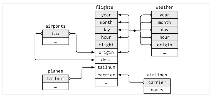
The key variables between flights and the other datasets are:
- flights dataset <- origin and dest both = faa -> airports dataset
- flights dataset <- tailnum -> planes dataset
- flights dataset <- origin, year, month, day, and hour -> weather dataset
- flights dataset <- carrier -> airlines dataset
8.4 Getting started
First, install the packages if you haven’t already done so (you probably installed dplyr in a previous lesson):
install.packages("dplyr")
install.packages("nycflights13")
Then, load the packages:
Let’s take a peek at the main nycflights13 dataset, “flights”:
flights# A tibble: 336,776 × 19
year month day dep_time sched_de…¹ dep_d…² arr_t…³ sched…⁴ arr_d…⁵ carrier
<int> <int> <int> <int> <int> <dbl> <int> <int> <dbl> <chr>
1 2013 1 1 517 515 2 830 819 11 UA
2 2013 1 1 533 529 4 850 830 20 UA
3 2013 1 1 542 540 2 923 850 33 AA
4 2013 1 1 544 545 -1 1004 1022 -18 B6
5 2013 1 1 554 600 -6 812 837 -25 DL
6 2013 1 1 554 558 -4 740 728 12 UA
7 2013 1 1 555 600 -5 913 854 19 B6
8 2013 1 1 557 600 -3 709 723 -14 EV
9 2013 1 1 557 600 -3 838 846 -8 B6
10 2013 1 1 558 600 -2 753 745 8 AA
# … with 336,766 more rows, 9 more variables: flight <int>, tailnum <chr>,
# origin <chr>, dest <chr>, air_time <dbl>, distance <dbl>, hour <dbl>,
# minute <dbl>, time_hour <dttm>, and abbreviated variable names
# ¹sched_dep_time, ²dep_delay, ³arr_time, ⁴sched_arr_time, ⁵arr_delayAnd get some more information about the flights dataset:
?flightsThis tells us that the airline name, as opposed to a two-letter carrier abbreviation,
can be found in the airlines dataset, and that the airports dataset gives
more information on the flight destinations.
First, we will drop some variables from flights to make our work more evident.
# A tibble: 336,776 × 9
    year month   day dep_delay carrier flight tailnum origin dest
   <int> <int> <int>     <dbl> <chr>    <int> <chr>   <chr>  <chr>
 1  2013     1     1         2 UA        1545 N14228  EWR    IAH
 2  2013     1     1         4 UA        1714 N24211  LGA    IAH
 3  2013     1     1         2 AA        1141 N619AA  JFK    MIA
 4  2013     1     1        -1 B6         725 N804JB  JFK    BQN
 5  2013     1     1        -6 DL         461 N668DN  LGA    ATL
 6  2013     1     1        -4 UA        1696 N39463  EWR    ORD
 7  2013     1     1        -5 B6         507 N516JB  EWR    FLL
 8  2013     1     1        -3 EV        5708 N829AS  LGA    IAD
 9  2013     1     1        -3 B6          79 N593JB  JFK    MCO
10  2013     1     1        -2 AA         301 N3ALAA  LGA    ORD
# … with 336,766 more rows
8.4.1 Data analysis questions
How would we answer the following questions:
what is the total number of flights per airline, but with the airline name showing instead of the carrier abbreviation?
how many flights occurred when the temperature fell below freezing?
are older planes more likely to have a delayed arrival?
Answering questions such as these requires us to join datasets.
8.5 Using left_join()
The syntax for dplyr joins is: xxx_join(x, y, by = "key_variable").
To answer the first question (i.e., number of flights per airline), we need to join the flights and airlines datasets. We want a left join because we want to add the airline names from airlines (as our second table) to flights (our first table). From above, we know that the flights dataset has a variable called ‘carrier’, and that that same variable is in the airlines dataset – this is our key (or “by” variable).
left_join(x = flights_mini, y = airlines, by = "carrier")# A tibble: 336,776 × 10
year month day dep_delay carrier flight tailnum origin dest name
<int> <int> <int> <dbl> <chr> <int> <chr> <chr> <chr> <chr>
1 2013 1 1 2 UA 1545 N14228 EWR IAH United Air L…
2 2013 1 1 4 UA 1714 N24211 LGA IAH United Air L…
3 2013 1 1 2 AA 1141 N619AA JFK MIA American Air…
4 2013 1 1 -1 B6 725 N804JB JFK BQN JetBlue Airw…
5 2013 1 1 -6 DL 461 N668DN LGA ATL Delta Air Li…
6 2013 1 1 -4 UA 1696 N39463 EWR ORD United Air L…
7 2013 1 1 -5 B6 507 N516JB EWR FLL JetBlue Airw…
8 2013 1 1 -3 EV 5708 N829AS LGA IAD ExpressJet A…
9 2013 1 1 -3 B6 79 N593JB JFK MCO JetBlue Airw…
10 2013 1 1 -2 AA 301 N3ALAA LGA ORD American Air…
# … with 336,766 more rowsWe can see that the number of rows has stayed the same: 366,776, but that we have one new column (at the end) called “name”.
Note that we could have instead used the pipe operator after summoning ‘flights_mini’.
# A tibble: 336,776 × 10
    year month   day dep_delay carrier flight tailnum origin dest  name
   <int> <int> <int>     <dbl> <chr>    <int> <chr>   <chr>  <chr> <chr>
 1  2013     1     1         2 UA        1545 N14228  EWR    IAH   United Air L…
 2  2013     1     1         4 UA        1714 N24211  LGA    IAH   United Air L…
 3  2013     1     1         2 AA        1141 N619AA  JFK    MIA   American Air…
 4  2013     1     1        -1 B6         725 N804JB  JFK    BQN   JetBlue Airw…
 5  2013     1     1        -6 DL         461 N668DN  LGA    ATL   Delta Air Li…
 6  2013     1     1        -4 UA        1696 N39463  EWR    ORD   United Air L…
 7  2013     1     1        -5 B6         507 N516JB  EWR    FLL   JetBlue Airw…
 8  2013     1     1        -3 EV        5708 N829AS  LGA    IAD   ExpressJet A…
 9  2013     1     1        -3 B6          79 N593JB  JFK    MCO   JetBlue Airw…
10  2013     1     1        -2 AA         301 N3ALAA  LGA    ORD   American Air…
# … with 336,766 more rowsNow, let’s wrangle to get the total counts, by grouping by either carrier or the new “name” variable brought in from the airlines dataset. Note that we can also drop the argument names (e.g., no “y” in “y = airlines”). I tend to keep the “by” argument name in to keep my code a bit more clear.
flights_mini %>%
  left_join(airlines, by = "carrier") %>%
  group_by(name) %>%
  summarize(total_flights = n())
# A tibble: 16 × 2
name total_flights
<chr> <int>
1 AirTran Airways Corporation 3260
2 Alaska Airlines Inc. 714
3 American Airlines Inc. 32729
4 Delta Air Lines Inc. 48110
5 Endeavor Air Inc. 18460
6 Envoy Air 26397
7 ExpressJet Airlines Inc. 54173
8 Frontier Airlines Inc. 685
9 Hawaiian Airlines Inc. 342
10 JetBlue Airways 54635
11 Mesa Airlines Inc. 601
12 SkyWest Airlines Inc. 32
13 Southwest Airlines Co. 12275
14 United Air Lines Inc. 58665
15 US Airways Inc. 20536
16 Virgin America 5162We can also rename variables within our join call. Let’s rename “name” to “airline” (and sort descending by number of flights).
flights_mini %>%
  left_join(airlines %>% select(carrier, Airline = name), by = "carrier") %>%
  ## make sure you use the new variable name
  group_by(Airline) %>%
  summarize(`Total Flights` = n()) %>%
  arrange(desc(`Total Flights`))
# A tibble: 16 × 2
Airline `Total Flights`
<chr> <int>
1 United Air Lines Inc. 58665
2 JetBlue Airways 54635
3 ExpressJet Airlines Inc. 54173
4 Delta Air Lines Inc. 48110
5 American Airlines Inc. 32729
6 Envoy Air 26397
7 US Airways Inc. 20536
8 Endeavor Air Inc. 18460
9 Southwest Airlines Co. 12275
10 Virgin America 5162
11 AirTran Airways Corporation 3260
12 Alaska Airlines Inc. 714
13 Frontier Airlines Inc. 685
14 Mesa Airlines Inc. 601
15 Hawaiian Airlines Inc. 342
16 SkyWest Airlines Inc. 328.5.1 Challenge 1 (2 minutes)
How would you add each plane’s manufacture year (rename it “manufacture_year”) to the flights dataset?
Solution to challenge 1
# A tibble: 336,776 × 10 year month day dep_delay carrier flight tailnum origin dest manufacture…¹ <int> <int> <int> <dbl> <chr> <int> <chr> <chr> <chr> <int> 1 2013 1 1 2 UA 1545 N14228 EWR IAH 1999 2 2013 1 1 4 UA 1714 N24211 LGA IAH 1998 3 2013 1 1 2 AA 1141 N619AA JFK MIA 1990 4 2013 1 1 -1 B6 725 N804JB JFK BQN 2012 5 2013 1 1 -6 DL 461 N668DN LGA ATL 1991 6 2013 1 1 -4 UA 1696 N39463 EWR ORD 2012 7 2013 1 1 -5 B6 507 N516JB EWR FLL 2000 8 2013 1 1 -3 EV 5708 N829AS LGA IAD 1998 9 2013 1 1 -3 B6 79 N593JB JFK MCO 2004 10 2013 1 1 -2 AA 301 N3ALAA LGA ORD NA # … with 336,766 more rows, and abbreviated variable name ¹manufacture_year## same as this: flights_mini %>% left_join(planes %>% select(tailnum, manufacture_year = year), by = "tailnum")# A tibble: 336,776 × 10 year month day dep_delay carrier flight tailnum origin dest manufacture…¹ <int> <int> <int> <dbl> <chr> <int> <chr> <chr> <chr> <int> 1 2013 1 1 2 UA 1545 N14228 EWR IAH 1999 2 2013 1 1 4 UA 1714 N24211 LGA IAH 1998 3 2013 1 1 2 AA 1141 N619AA JFK MIA 1990 4 2013 1 1 -1 B6 725 N804JB JFK BQN 2012 5 2013 1 1 -6 DL 461 N668DN LGA ATL 1991 6 2013 1 1 -4 UA 1696 N39463 EWR ORD 2012 7 2013 1 1 -5 B6 507 N516JB EWR FLL 2000 8 2013 1 1 -3 EV 5708 N829AS LGA IAD 1998 9 2013 1 1 -3 B6 79 N593JB JFK MCO 2004 10 2013 1 1 -2 AA 301 N3ALAA LGA ORD NA # … with 336,766 more rows, and abbreviated variable name ¹manufacture_year
One thing we haven’t specifically noted is that mutating joins will bring in all
variables from the matching dataset. You’ll see from the solution above that we
can change that behaviour by using select() and listing only those variables we
want to join in (don’t forget the key variable!).
8.6 Modifying the by argument
8.6.1 Excluding the by argument
We can modify the “by” argument a few ways. See what happens if we don’t
specify a by variable.
## joining without specifying a `by` variable
left_join(flights_mini, airlines)
Joining, by = "carrier"# A tibble: 336,776 × 10
year month day dep_delay carrier flight tailnum origin dest name
<int> <int> <int> <dbl> <chr> <int> <chr> <chr> <chr> <chr>
1 2013 1 1 2 UA 1545 N14228 EWR IAH United Air L…
2 2013 1 1 4 UA 1714 N24211 LGA IAH United Air L…
3 2013 1 1 2 AA 1141 N619AA JFK MIA American Air…
4 2013 1 1 -1 B6 725 N804JB JFK BQN JetBlue Airw…
5 2013 1 1 -6 DL 461 N668DN LGA ATL Delta Air Li…
6 2013 1 1 -4 UA 1696 N39463 EWR ORD United Air L…
7 2013 1 1 -5 B6 507 N516JB EWR FLL JetBlue Airw…
8 2013 1 1 -3 EV 5708 N829AS LGA IAD ExpressJet A…
9 2013 1 1 -3 B6 79 N593JB JFK MCO JetBlue Airw…
10 2013 1 1 -2 AA 301 N3ALAA LGA ORD American Air…
# … with 336,766 more rowsR will match by any variable with the same name in both datasets. Be careful - this might not be what you want!
left_join(flights_mini, planes)Joining, by = c("year", "tailnum")# A tibble: 336,776 × 16
year month day dep_delay carrier flight tailnum origin dest type manuf…¹
<int> <int> <int> <dbl> <chr> <int> <chr> <chr> <chr> <chr> <chr>
1 2013 1 1 2 UA 1545 N14228 EWR IAH <NA> <NA>
2 2013 1 1 4 UA 1714 N24211 LGA IAH <NA> <NA>
3 2013 1 1 2 AA 1141 N619AA JFK MIA <NA> <NA>
4 2013 1 1 -1 B6 725 N804JB JFK BQN <NA> <NA>
5 2013 1 1 -6 DL 461 N668DN LGA ATL <NA> <NA>
6 2013 1 1 -4 UA 1696 N39463 EWR ORD <NA> <NA>
7 2013 1 1 -5 B6 507 N516JB EWR FLL <NA> <NA>
8 2013 1 1 -3 EV 5708 N829AS LGA IAD <NA> <NA>
9 2013 1 1 -3 B6 79 N593JB JFK MCO <NA> <NA>
10 2013 1 1 -2 AA 301 N3ALAA LGA ORD <NA> <NA>
# … with 336,766 more rows, 5 more variables: model <chr>, engines <int>,
# seats <int>, speed <int>, engine <chr>, and abbreviated variable name
# ¹manufacturerThe variable “year” exists in both flights_mini and planes, but means different things. When not specifying the key, R assumed you wanted to join by “year” as well, which resulted in a lot of NAs!
8.6.2 Joining on multiple keys
You may have noticed earlier that we can join by more than one variable. To do
so, simply use c("variable1", "variable2", "etc") for your keys. Notice that
year, month, day, and origin are in both the flights_mini and weather datasets.
# A tibble: 8,036,575 × 20
    year month   day dep_delay carrier flight tailnum origin dest   hour  temp
   <int> <int> <int>     <dbl> <chr>    <int> <chr>   <chr>  <chr> <int> <dbl>
 1  2013     1     1         2 UA        1545 N14228  EWR    IAH       1  39.0
 2  2013     1     1         2 UA        1545 N14228  EWR    IAH       2  39.0
 3  2013     1     1         2 UA        1545 N14228  EWR    IAH       3  39.0
 4  2013     1     1         2 UA        1545 N14228  EWR    IAH       4  39.9
 5  2013     1     1         2 UA        1545 N14228  EWR    IAH       5  39.0
 6  2013     1     1         2 UA        1545 N14228  EWR    IAH       6  37.9
 7  2013     1     1         2 UA        1545 N14228  EWR    IAH       7  39.0
 8  2013     1     1         2 UA        1545 N14228  EWR    IAH       8  39.9
 9  2013     1     1         2 UA        1545 N14228  EWR    IAH       9  39.9
10  2013     1     1         2 UA        1545 N14228  EWR    IAH      10  41
# … with 8,036,565 more rows, and 9 more variables: dewp <dbl>, humid <dbl>,
#   wind_dir <dbl>, wind_speed <dbl>, wind_gust <dbl>, precip <dbl>,
#   pressure <dbl>, visib <dbl>, time_hour <dttm>
You’ll see that we now have over 8 million rows. This is because the “hour” variable in weather matched many times for each year X month X day X origin combination, resulting in repeat of information from flights_mini.
What happens if you didn’t know that “year” was in both datasets?
# A tibble: 8,036,575 × 21
   year.x month   day dep_delay carrier flight tailnum origin dest  year.y  hour
    <int> <int> <int>     <dbl> <chr>    <int> <chr>   <chr>  <chr>  <int> <int>
 1   2013     1     1         2 UA        1545 N14228  EWR    IAH     2013     1
 2   2013     1     1         2 UA        1545 N14228  EWR    IAH     2013     2
 3   2013     1     1         2 UA        1545 N14228  EWR    IAH     2013     3
 4   2013     1     1         2 UA        1545 N14228  EWR    IAH     2013     4
 5   2013     1     1         2 UA        1545 N14228  EWR    IAH     2013     5
 6   2013     1     1         2 UA        1545 N14228  EWR    IAH     2013     6
 7   2013     1     1         2 UA        1545 N14228  EWR    IAH     2013     7
 8   2013     1     1         2 UA        1545 N14228  EWR    IAH     2013     8
 9   2013     1     1         2 UA        1545 N14228  EWR    IAH     2013     9
10   2013     1     1         2 UA        1545 N14228  EWR    IAH     2013    10
# … with 8,036,565 more rows, and 10 more variables: temp <dbl>, dewp <dbl>,
#   humid <dbl>, wind_dir <dbl>, wind_speed <dbl>, wind_gust <dbl>,
#   precip <dbl>, pressure <dbl>, visib <dbl>, time_hour <dttm>
The “year” variable from flights_mini has been renamed “year.x”, and “year” from “weather” has been renamed “year.y”. (Whenever this happens, variables ending in “.x” come from the first table, while those ending in “.y” come from the other table.)
8.6.3 Key variables with different names
We can also match on a key that has a different name in the related tables (although its values are the same). The variable “faa” in airports is equivalent to flights_mini’s “dest” variable. Here are three ways of getting the same result.
# A tibble: 336,776 × 16
    year month   day dep_delay carrier flight tailnum origin dest  name      lat
   <int> <int> <int>     <dbl> <chr>    <int> <chr>   <chr>  <chr> <chr>   <dbl>
 1  2013     1     1         2 UA        1545 N14228  EWR    IAH   George…  30.0
 2  2013     1     1         4 UA        1714 N24211  LGA    IAH   George…  30.0
 3  2013     1     1         2 AA        1141 N619AA  JFK    MIA   Miami …  25.8
 4  2013     1     1        -1 B6         725 N804JB  JFK    BQN   <NA>     NA
 5  2013     1     1        -6 DL         461 N668DN  LGA    ATL   Hartsf…  33.6
 6  2013     1     1        -4 UA        1696 N39463  EWR    ORD   Chicag…  42.0
 7  2013     1     1        -5 B6         507 N516JB  EWR    FLL   Fort L…  26.1
 8  2013     1     1        -3 EV        5708 N829AS  LGA    IAD   Washin…  38.9
 9  2013     1     1        -3 B6          79 N593JB  JFK    MCO   Orland…  28.4
10  2013     1     1        -2 AA         301 N3ALAA  LGA    ORD   Chicag…  42.0
# … with 336,766 more rows, and 5 more variables: lon <dbl>, alt <dbl>,
# tz <dbl>, dst <chr>, tzone <chr># A tibble: 336,776 × 16
year month day dep_delay carrier flight tailnum origin dest name lat
<int> <int> <int> <dbl> <chr> <int> <chr> <chr> <chr> <chr> <dbl>
1 2013 1 1 2 UA 1545 N14228 EWR IAH George… 30.0
2 2013 1 1 4 UA 1714 N24211 LGA IAH George… 30.0
3 2013 1 1 2 AA 1141 N619AA JFK MIA Miami … 25.8
4 2013 1 1 -1 B6 725 N804JB JFK BQN <NA> NA
5 2013 1 1 -6 DL 461 N668DN LGA ATL Hartsf… 33.6
6 2013 1 1 -4 UA 1696 N39463 EWR ORD Chicag… 42.0
7 2013 1 1 -5 B6 507 N516JB EWR FLL Fort L… 26.1
8 2013 1 1 -3 EV 5708 N829AS LGA IAD Washin… 38.9
9 2013 1 1 -3 B6 79 N593JB JFK MCO Orland… 28.4
10 2013 1 1 -2 AA 301 N3ALAA LGA ORD Chicag… 42.0
# … with 336,766 more rows, and 5 more variables: lon <dbl>, alt <dbl>,
# tz <dbl>, dst <chr>, tzone <chr>Joining, by = "dest"# A tibble: 336,776 × 16
year month day dep_delay carrier flight tailnum origin dest name lat
<int> <int> <int> <dbl> <chr> <int> <chr> <chr> <chr> <chr> <dbl>
1 2013 1 1 2 UA 1545 N14228 EWR IAH George… 30.0
2 2013 1 1 4 UA 1714 N24211 LGA IAH George… 30.0
3 2013 1 1 2 AA 1141 N619AA JFK MIA Miami … 25.8
4 2013 1 1 -1 B6 725 N804JB JFK BQN <NA> NA
5 2013 1 1 -6 DL 461 N668DN LGA ATL Hartsf… 33.6
6 2013 1 1 -4 UA 1696 N39463 EWR ORD Chicag… 42.0
7 2013 1 1 -5 B6 507 N516JB EWR FLL Fort L… 26.1
8 2013 1 1 -3 EV 5708 N829AS LGA IAD Washin… 38.9
9 2013 1 1 -3 B6 79 N593JB JFK MCO Orland… 28.4
10 2013 1 1 -2 AA 301 N3ALAA LGA ORD Chicag… 42.0
# … with 336,766 more rows, and 5 more variables: lon <dbl>, alt <dbl>,
# tz <dbl>, dst <chr>, tzone <chr>8.7 Other mutating joins
We have only been working with left joins so far. The idea is exactly the same for full, right and inner joins.
full_join(x, y, by)- everything!right_join(x, y, by)- equivalent to left_join(y, x, by), but the columns and rows will be ordered differentlyinner_join(x, y, by)- only rows found in both
The difference is what you end up with.
Let’s create two small datasets to compare the results of the above types of joins. Both tables have an ID column – this is our key – and one other variable.
tbl1 <- tibble(ID = c("ID_1", "ID_2", "ID_3", "ID_4", "ID_5", "ID_6"),
              activity1 = c("cycling", "basketball", "kung fu", "reading", "running", "skating"))
tbl2 <- tibble(ID = c("ID_2", "ID_4", "ID_6", "ID_8"),
              place2 = c("outside court", "library", "rec center", "pool"))

tbl1
# A tibble: 6 × 2
ID activity1
<chr> <chr>
1 ID_1 cycling
2 ID_2 basketball
3 ID_3 kung fu
4 ID_4 reading
5 ID_5 running
6 ID_6 skating
tbl2# A tibble: 4 × 2
ID place2
<chr> <chr>
1 ID_2 outside court
2 ID_4 library
3 ID_6 rec center
4 ID_8 pool
left_join(tbl1, tbl2, by = "ID")# A tibble: 6 × 3
ID activity1 place2
<chr> <chr> <chr>
1 ID_1 cycling <NA>
2 ID_2 basketball outside court
3 ID_3 kung fu <NA>
4 ID_4 reading library
5 ID_5 running <NA>
6 ID_6 skating rec center
right_join(tbl2, tbl1, by = "ID")# A tibble: 6 × 3
ID place2 activity1
<chr> <chr> <chr>
1 ID_2 outside court basketball
2 ID_4 library reading
3 ID_6 rec center skating
4 ID_1 <NA> cycling
5 ID_3 <NA> kung fu
6 ID_5 <NA> running
right_join(tbl1, tbl2, by = "ID")# A tibble: 4 × 3
ID activity1 place2
<chr> <chr> <chr>
1 ID_2 basketball outside court
2 ID_4 reading library
3 ID_6 skating rec center
4 ID_8 <NA> pool
full_join(tbl1, tbl2, by = "ID")# A tibble: 7 × 3
ID activity1 place2
<chr> <chr> <chr>
1 ID_1 cycling <NA>
2 ID_2 basketball outside court
3 ID_3 kung fu <NA>
4 ID_4 reading library
5 ID_5 running <NA>
6 ID_6 skating rec center
7 ID_8 <NA> pool
inner_join(tbl1, tbl2, by = "ID")# A tibble: 3 × 3
ID activity1 place2
<chr> <chr> <chr>
1 ID_2 basketball outside court
2 ID_4 reading library
3 ID_6 skating rec center 8.7.1 Challenge 2 (5 minutes)
How many flights occurred when the temperature fell below freezing?
Hint: use the
group_by()andsummarize()functions we learned in thedplyrlesson.Solution to challenge 2
## first, find the days where the temperature fell below 32 F (freezing)
freezing <- weather %>%
  group_by(month, day) %>%
  summarize(mean_temp = mean(temp, na.rm = TRUE), .groups = "drop") %>%
  filter(mean_temp < 32)

## inner join to get only days with freezing temperature
flights_mini %>% inner_join(freezing, by = c("month", "day")) ## number of rows
# A tibble: 29,116 × 10 year month day dep_delay carrier flight tailnum origin dest mean_temp <int> <int> <int> <dbl> <chr> <int> <chr> <chr> <chr> <dbl> 1 2013 1 2 43 B6 707 N580JB JFK SJU 28.7 2 2013 1 2 156 B6 22 N636JB JFK SYR 28.7 3 2013 1 2 -2 US 1030 N162UW EWR CLT 28.7 4 2013 1 2 -3 UA 1453 N76515 EWR IAH 28.7 5 2013 1 2 -5 AA 1141 N621AA JFK MIA 28.7 6 2013 1 2 7 UA 407 N493UA LGA IAH 28.7 7 2013 1 2 -6 B6 725 N624JB JFK BQN 28.7 8 2013 1 2 -6 B6 125 N637JB JFK FLL 28.7 9 2013 1 2 -6 B6 49 N658JB JFK PBI 28.7 10 2013 1 2 -6 B6 371 N805JB LGA FLL 28.7 # … with 29,106 more rowsflights_mini %>% inner_join(freezing) %>% tally() ## or, get the numberJoining, by = c("month", "day")# A tibble: 1 × 1 n <int> 1 29116
8.8 Filtering joins
In Challenge 2, we could have done a semi join instead of an inner join. That is, we were essentially filtering the ‘flights_mini’ dataset to get only those flights that occurred on days where the average temperature was below 32F. We didn’t do anything with the actual temperature other than drop observations; therefore, we didn’t actually need the ‘mean_temp’ variable.
# A tibble: 29,116 × 9
    year month   day dep_delay carrier flight tailnum origin dest
   <int> <int> <int>     <dbl> <chr>    <int> <chr>   <chr>  <chr>
 1  2013     1     2        43 B6         707 N580JB  JFK    SJU
 2  2013     1     2       156 B6          22 N636JB  JFK    SYR
 3  2013     1     2        -2 US        1030 N162UW  EWR    CLT
 4  2013     1     2        -3 UA        1453 N76515  EWR    IAH
 5  2013     1     2        -5 AA        1141 N621AA  JFK    MIA
 6  2013     1     2         7 UA         407 N493UA  LGA    IAH
 7  2013     1     2        -6 B6         725 N624JB  JFK    BQN
 8  2013     1     2        -6 B6         125 N637JB  JFK    FLL
 9  2013     1     2        -6 B6          49 N658JB  JFK    PBI
10  2013     1     2        -6 B6         371 N805JB  LGA    FLL
# … with 29,106 more rows
That is what happens with filtering joins: observations from one table are
filtered based on whether or not they match an observation in the other table,
but no information is brought in from the other table. Specifically, semi joins
return all rows in x with a match in y, while anti joins return all rows in x
without a match in y. Note, that the syntax for filtering joins is the same:
xxx_join(x, y, by = "key_variable").