11 Data analysis reports
Data analysts tend to write a lot of reports, describing their analyses and results, for their collaborators or to document their work for future reference.
Many new users begin by first writing a single R script containing all of the work. Then simply share the analysis by emailing the script and various graphs as attachments. But this can be cumbersome, requiring a lengthy discussion to explain which attachment was which result.
Writing formal reports with Word or LaTeX can simplify this by incorporating both the analysis report and output graphs into a single document. But tweaking formatting to make figures look correct and fix obnoxious page breaks can be tedious and lead to a lengthly “whack a mole” game of fixing new mistakes resulting from a single formatting change.
Creating a web page (as an html file) by using R Markdown makes things easier. The report can be one long stream, so tall figures that wouldn’t ordinary fit on one page can be kept full size and easier to read, since the reader can simply keep scrolling. Formatting is simple and easy to modify, allowing you to spend more time on your analyses instead of writing reports.
11.1 Literate programming
Ideally, such analysis reports are reproducible documents: If an error is discovered, or if some additional subjects are added to the data, you can just re-compile the report and get the new or corrected results (versus having to reconstruct figures, paste them into a Word document, and further hand-edit various detailed results).
The key R package is knitr. It allows you
to create a document that is a mixture of text and chunks of
code. When the document is processed by knitr, chunks of code will
be executed, and graphs or other results inserted into the final document.
This sort of idea has been called “literate programming”.
knitr allows you to mix basically any sort of text with code from different programming languages, but we recommend that you use R Markdown, which mixes Markdown
with R. Markdown is a light-weight mark-up language for documents and web pages.
11.2 Example of Using R Markdown in the BC Government
R Markdown is quite versatile. Below are some examples of ways you can adapt it for a variety of purposes.
11.2.3 Presentation
- Rendered: https://bcgov.github.io/bcgov-rstats-public-presentations/2020-03-26_bcdata_lunch_and_learn/bcdata-2020-lunch-and-learn.html#1
- R Markdown: https://github.com/bcgov/bcgov-rstats-public-presentations/blob/master/2020-03-26_bcdata_lunch_and_learn/bcdata-2020-lunch-and-learn.Rmd
Challenge 1 (5 minutes)
Take a few minutes to discuss in your groups the typical ways in which you share results. What you do you do in the scenario where the data changes but the analysis needs to be the same?
11.3 Creating an R Markdown file
Within RStudio, click File → New File → R Markdown and you’ll get a dialog box like this:
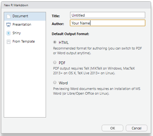
You can stick with the default (HTML output), but give it a title and an author=.
11.4 Basic components of R Markdown
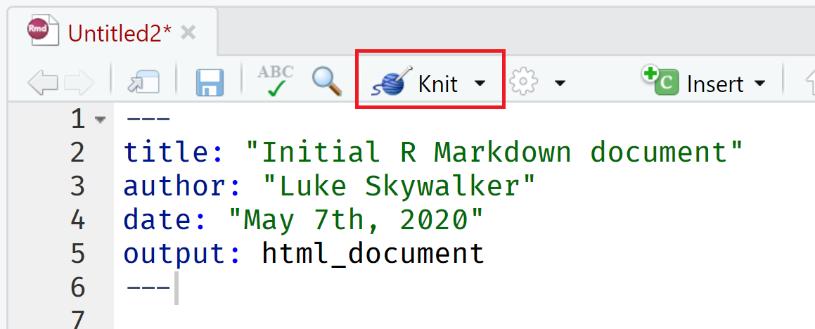
The initial chunk of text (header) contains instructions for R to specify what kind of document will be created, and the options chosen. You can use the header to give your document a title, author, date, and tell it that you’re going to want to produce html output (in other words, a web page).
---
title: "Initial R Markdown document"
author: "Luke Skywalker"
date: "May 7th, 2020"
output: html_document
---
You can delete any of those fields if you don’t want them included. The double-quotes aren’t strictly necessary in this case. They’re mostly needed if you want to include a colon in the title.
RStudio creates the document with some example text to get you started. Note below that there are chunks like
```{r}
summary(cars)
```
These are chunks of R code that will be executed by knitr and replaced
by their results. More on this later.
Also note the web address that’s put between angle brackets (< >) as
well as the double-asterisks in **Knit**. This is
Markdown.
11.5 Markdown
Markdown is a system for writing web pages by marking up the text much as you would in an email rather than writing html code. The marked-up text gets converted to html, replacing the marks with the proper html code.
For now, let’s delete all of the stuff that’s there and write a bit of markdown.
You make things bold using two asterisks, like this: **bold**,
and you make things italics by using underscores, like this:
_italics_.
You can make a bulleted list by writing a list with hyphens or asterisks, like this:
* bold with double-asterisks
* italics with underscores
* code-type font with backticks
or like this:
- bold with double-asterisks
- italics with underscores
- code-type font with backticks
Each will appear as:
- bold with double-asterisks
- italics with underscores
- code-type font with backticks
You can use whatever method you prefer, but be consistent. This maintains the readability of your code.
You can make a numbered list by just using numbers. You can even use the same number over and over if you want:
1. bold with double-asterisks
1. italics with underscores
1. code-type font with backticks
This will appear as:
- bold with double-asterisks
- italics with underscores
- code-type font with backticks
You can make section headers of different sizes by initiating a line
with some number of # symbols:
# Title
## Main section
### Sub-section
#### Sub-sub section
You compile the R Markdown document to an html webpage by clicking the “Knit” button in the upper-left.
Challenge 2
Create a new R Markdown document. Delete all of the R code chunks and write a bit of Markdown (some sections, some italicized text, and an itemized list).
Convert the document to a webpage.
Solution to Challenge 2
In RStudio, select File > New file > R Markdown…
Delete the placeholder text and add the following:
# Introduction

## Background on Data

This report uses the *gapminder* dataset, which has columns that include:

* country
* continent
* year
* lifeExp
* pop
* gdpPercap

## Background on Methods
Then click the ‘Knit’ button on the toolbar to generate an html document (webpage).
11.5.1 A bit more Markdown
You can make a hyperlink like this:
[text to show](http://the-web-page.com).
You can include an image file like this: 
You can do subscripts (e.g., F2) with F~2~ and superscripts (e.g.,
F2) with F^2^.
If you know how to write equations in
LaTeX, you can use $ $ and $$ $$ to insert math equations, like
$E = mc^2$ and
$$y = \mu + \sum_{i=1}^p \beta_i x_i + \epsilon$$You can review Markdown syntax by navigating to the “Markdown Quick Reference” under the “Help” field in the toolbar at the top of RStudio.
11.5.2 R code chunks
The real power of Markdown comes from mixing markdown with chunks of code. This is R Markdown. When processed, the R code will be executed; if they produce figures, the figures will be inserted in the final document.
The main code chunks look like this:
```{r load_data}
library("readr")
gapminder
That is, you place a chunk of R code between ```{r chunk_name}
and ```. You should give each chunk
a unique name, as they will help you to fix errors and, if any graphs are
produced, the file names are based on the name of the code chunk that
produced them.
11.6 How R Markdown gets compiled
When you press the “Knit” button knitr will process your R Markdown file to create a plain Markdown document (along with a set of figure files if needed).
If we specified our output document to be a html file, the Markdown file (and figure documents) is then converted or rendered to a html file using the tool pandoc.
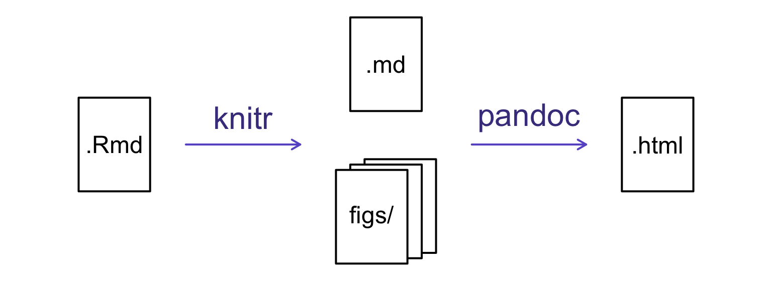
Different output document types require different tool for conversion. This will be discused below.
11.7 Chunk options
As we saw above, code chunks are a very important part of using R Markdown. We will now explore some of the options for controlling how these will show up in our document.
Firstly we need name our code chunk name. By default all code chunks are blank. ie:
```{r}
```
It is recomended to use a descriptive name such as’load_data’ or ‘read_libraries’. This will help you break up your code chunks and ensure each chunk has a unique name.
```{r load_libraries}
library("dplyr")
library("ggplot2")
```
We can control how the code and the resulting outputs are shown in the final output by changing the code chunk options which follow the title. For example:
```{r load_libraries, eval = FALSE, echo = TRUE}
library("dplyr")
library("ggplot2")
```
There are many different options you can adjust. More details can be found on the R Markdown cheatsheet or here.
The ones you need to know first are:
-
cache: TRUE/FALSE. Do you want the output of the chunk saved so you dont have to run it next time? -
eval: Do you want to code to be evaluated? -
echo: Do you want to print the code? -
include: Do you want to include the code in the output document? -
warning=FALSEandmessage=FALSE: Do you want to hide any warnings or messages? -
fig.heightandfig.width: Do you want to set figures sizes (inches)?
Tips: Finding help with chunk options You can review all of the
Rchunk options by navigating to the “R Markdown Cheat Sheet” under the “Cheatsheets” section of the “Help” field in the toolbar at the top of RStudio.
Lets create a code chunk. Firstly add a name addup and set the eval parameter to TRUE.
```{r addup, eval = TRUE}
1 + 1
```
When we knit the document we can see both the code and the result:
1 + 1 [1] 2If we dont want the code to appear in the output we can use the echo parameters.
```{r addup, eval = TRUE, echo = FALSE}
1 + 1
```
When knit the document will now only show the result and will hide the code.
[1] 211.7.1 Global options
Often there will be particular options that you’ll want to use repeatedly; for this, you can set global chunk options, like so:
```{r global_options, echo=FALSE}
knitr::opts_chunk$set(fig.path="Figs/",
                      message=FALSE,
                      warning=FALSE,
                      echo=FALSE,
                      results="hide",
                      fig.width=11)
```
11.7.2 Formatting figures
We can use paramaters to control the location and size of plots using fig.height,fig.width
and fig.align. We can also use fig.cap to add a title.
We can use the gapminder dataset and ggplot2package to create and format a plot within R Markdown.
```{r pretty_plot, eval = TRUE, echo = FALSE, fig.cap = "A nice descriptive title"}
library("readr")
library("ggplot2")
gapminder
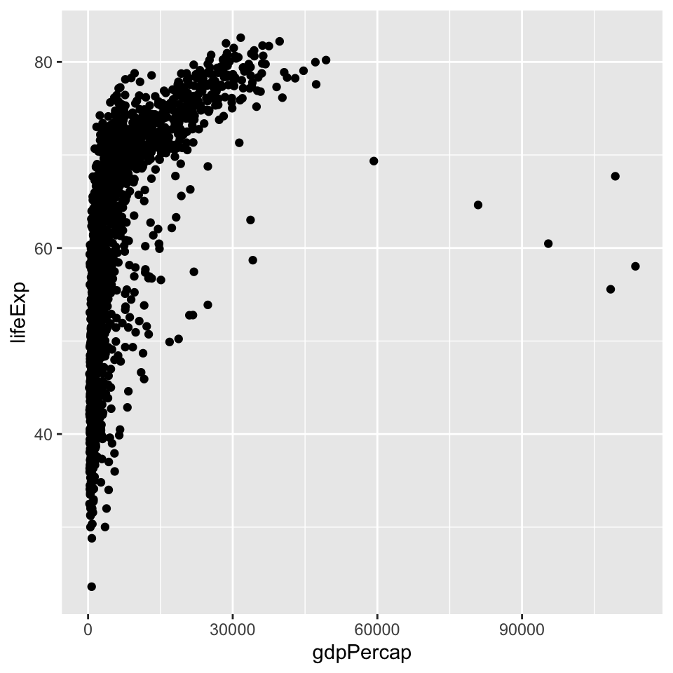
Figure 11.1: A nice descriptive title
Challenge 4
Generate a plot using the gapminder dataset and ggplot2 package. Use the chunk options to control the size and alignment of the figure.
Solution to Challenge 4
```{r pretty_plot, eval = TRUE, echo = FALSE, fig.cap= "Pretty Plot", fig.width = 5, fig.height = 5, fig.align = 'centre'}
ggplot(data = gapminder, mapping = aes(x = gdpPercap, y = lifeExp)) +
geom_point()
```

(#fig:pretty_plot)Pretty Plot
11.8 Inline R code
To make your document reproducible, you can also use r to populate values within a sentence. This will ensure values are automatically updated. We can use `r and ` to designate in-line code.
For example: `r round( value, 2)`. The code will be
executed and replaced with the evaluated value as the result.
For example:
`r round(3.141593, 2)` will show as
3.14
This is useful when incorporating data or calculations directly into a sentence:
The ratio of a circle’s circumference to its diameter is `r round(3.141593, 2) `.
This will appear as:
The ratio of a circle's circumference to its diameter is 3.14
We can also do calculations on the fly within our inline code. For example we can calculate the number of instructors and populate a sentence. Firstly lets use length() to determine the number of instructors:
` r length(c(“Andy”, “Gen”, “Sam”, “Steph”))`
when we run this in the R console we should get 4.
Now we can add this as in-line code by using `r and ` :
this course has ` r length(c(“Andy”, “Gen”, “Sam”, “Steph”))` instructors
The rendered fomat will look like
this course has 4 instructors
Challenge 5
Try out a bit of in-line R code using a simple addition eg: 2+2.
Solution to Challenge 5
Here’s some inline code to determine that 2 + 2 =
4.
11.9 Other outputs: Word, PDF and more…
We can convert R Markdown to a PDF or a Word document. Click the little triangle next to the “Knit” button to get a drop-down menu.
Alternatively we can change the YAML:
---
title: "Exploring R Markdown"
output: html_document
---
---
title: "Exploring R Markdown"
output: word_document
------
title: "Exploring R Markdown"
output: pdf_document
---11.9.1 A note about Rmd outputs
It can be easy to get caught up with how your document looks. It is highly recommended to render as html document and avoiding compiling to PDF or word until you really need to. This is also recommended by the author of rmarkdown and knitr, Yihui Xie. This means that you can spend time working on generating content, and not trying to get figures to line up correctly and wrestling with LaTex libraries.
Tips: Creating PDF documents
Markdown documents can be compiled to PDF, however it will likely you will require additional software called LaTex. This software can be tricky to install and it is reccommended to use
tinytex as an alternative. This R package is a lightweight version of LaTex is designed for r users. You can install using the following commands:tinytex::install_tinytex()There is lots of information and help available - see tinytex FQA page