7 Create Tidy Data with tidyr
People who work with data often want to reshape their dataframes from ‘wide’ to ‘longer’ layouts, or vice-versa. The ‘long’ layout or format is where:
- each column is a variable
- each row is an observation
In the purely ‘long’ (or ‘longest’) format, you usually have 1 column for the observed variable and the other columns are ID variables.
For the ‘wide’ format each row is often a site/subject/patient and you have
multiple observation variables containing the same type of data. These can be
either repeated observations over time, or observation of multiple variables (or
a mix of both). You may find data input may be simpler or some other
applications may prefer the ‘wide’ format. However, many of R‘s functions have
been designed assuming you have ’longer’ formatted data. This tutorial will help you
efficiently transform your data shape regardless of original format.
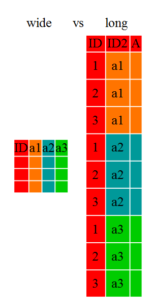
Long and wide dataframe layouts mainly affect readability. For humans, the wide format is often more intuitive since we can often see more of the data on the screen due to its shape. However, the long format is more machine readable and is closer to the formatting of databases. The ID variables in our dataframes are similar to the fields in a database and observed variables are like the database values.
7.1 Getting started
First install the packages if you haven’t already done so (you probably installed dplyr in the previous lesson):
install.packages("tidyr")
install.packages("dplyr")
Load the packages
First, lets look at the structure of our original gapminder dataframe:
gapminder <- read_csv("data/gapminder_data.csv")Rows: 1704 Columns: 6
── Column specification ────────────────────────────────────────────────────────
Delimiter: ","
chr (2): country, continent
dbl (4): year, pop, lifeExp, gdpPercap
ℹ Use `spec()` to retrieve the full column specification for this data.
ℹ Specify the column types or set `show_col_types = FALSE` to quiet this message.
gapminder# A tibble: 1,704 × 6
country year pop continent lifeExp gdpPercap
<chr> <dbl> <dbl> <chr> <dbl> <dbl>
1 Afghanistan 1952 8425333 Asia 28.8 779.
2 Afghanistan 1957 9240934 Asia 30.3 821.
3 Afghanistan 1962 10267083 Asia 32.0 853.
4 Afghanistan 1967 11537966 Asia 34.0 836.
5 Afghanistan 1972 13079460 Asia 36.1 740.
6 Afghanistan 1977 14880372 Asia 38.4 786.
7 Afghanistan 1982 12881816 Asia 39.9 978.
8 Afghanistan 1987 13867957 Asia 40.8 852.
9 Afghanistan 1992 16317921 Asia 41.7 649.
10 Afghanistan 1997 22227415 Asia 41.8 635.
# … with 1,694 more rows7.1.1 Challenge 1
Is gapminder a purely long, purely wide, or some intermediate format?
Solution to challenge 1
The original gapminder data.frame is in an intermediate format. It is not purely long since it had multiple observation variables (pop,lifeExp,gdpPercap).
Sometimes, as with the gapminder dataset, we have multiple types of observed
data. It is somewhere in between the purely ‘long’ and ‘wide’ data formats. We
have 3 “ID variables” (continent, country, year) and 3 “Observation
variables” (pop,lifeExp,gdpPercap). This intermediate format can be
preferred despite not having ALL observations in 1 column given that all 3
observation variables have different units. There are few operations that would
need us to make this dataframe any longer (i.e. 4 ID variables and 1
Observation variable).
While using many of the functions in R, which are often vector based, you
usually do not want to do mathematical operations on values with different
units. For example, using the purely long format, a single mean for all of the
values of population, life expectancy, and GDP would not be meaningful since it
would return the mean of values with 3 incompatible units. The solution is that
we first manipulate the data either by grouping (see the lesson on dplyr), or
we change the structure of the dataframe. Note: Some plotting functions in
R actually work better in the wide format data.
7.2 From wide to long format with pivot_longer()
Until now, we’ve been using the nicely formatted original gapminder dataset, but ‘real’ data (i.e. our own research data) will never be so well organized. Here let’s start with the wide formatted version of the gapminder dataset.
We’ll load the data file and look at it.
gap_wide <- read_csv("data/gapminder_wide.csv")Rows: 142 Columns: 38
── Column specification ────────────────────────────────────────────────────────
Delimiter: ","
chr (2): continent, country
dbl (36): pop_1952, lifeExp_1952, gdpPercap_1952, pop_1957, lifeExp_1957, gd...
ℹ Use `spec()` to retrieve the full column specification for this data.
ℹ Specify the column types or set `show_col_types = FALSE` to quiet this message.
gap_wide# A tibble: 142 × 38
continent country pop_1…¹ lifeE…² gdpPe…³ pop_1…⁴ lifeE…⁵ gdpPe…⁶ pop_1…⁷
<chr> <chr> <dbl> <dbl> <dbl> <dbl> <dbl> <dbl> <dbl>
1 Asia Afghanistan 8.43e6 28.8 779. 9.24e6 30.3 821. 1.03e7
2 Europe Albania 1.28e6 55.2 1601. 1.48e6 59.3 1942. 1.73e6
3 Africa Algeria 9.28e6 43.1 2449. 1.03e7 45.7 3014. 1.10e7
4 Africa Angola 4.23e6 30.0 3521. 4.56e6 32.0 3828. 4.83e6
5 Americas Argentina 1.79e7 62.5 5911. 1.96e7 64.4 6857. 2.13e7
6 Oceania Australia 8.69e6 69.1 10040. 9.71e6 70.3 10950. 1.08e7
7 Europe Austria 6.93e6 66.8 6137. 6.97e6 67.5 8843. 7.13e6
8 Asia Bahrain 1.20e5 50.9 9867. 1.39e5 53.8 11636. 1.72e5
9 Asia Bangladesh 4.69e7 37.5 684. 5.14e7 39.3 662. 5.68e7
10 Europe Belgium 8.73e6 68 8343. 8.99e6 69.2 9715. 9.22e6
# … with 132 more rows, 29 more variables: lifeExp_1962 <dbl>,
# gdpPercap_1962 <dbl>, pop_1967 <dbl>, lifeExp_1967 <dbl>,
# gdpPercap_1967 <dbl>, pop_1972 <dbl>, lifeExp_1972 <dbl>,
# gdpPercap_1972 <dbl>, pop_1977 <dbl>, lifeExp_1977 <dbl>,
# gdpPercap_1977 <dbl>, pop_1982 <dbl>, lifeExp_1982 <dbl>,
# gdpPercap_1982 <dbl>, pop_1987 <dbl>, lifeExp_1987 <dbl>,
# gdpPercap_1987 <dbl>, pop_1992 <dbl>, lifeExp_1992 <dbl>, …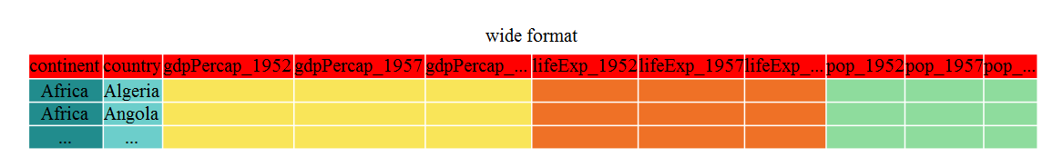
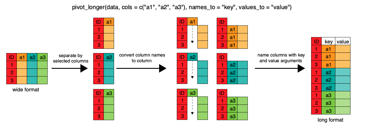
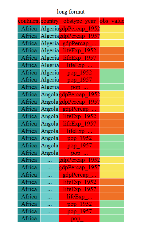
To change this very wide dataframe layout back to our nice, intermediate (or longer) layout, we will use one of the two available pivot functions from the tidyr package. To convert from wide to a longer format, we will use the pivot_longer() function. pivot_longer() makes datasets longer by increasing the number of rows and decreasing the number of columns, or ‘lengthening’ your observation variables into a single variable.
gap_long <- gap_wide %>%
  pivot_longer(
    cols = pop_1952:gdpPercap_2007,
    names_to = "obstype_year", values_to = "obs_values"
  )
gap_long
# A tibble: 5,112 × 4
continent country obstype_year obs_values
<chr> <chr> <chr> <dbl>
1 Asia Afghanistan pop_1952 8425333
2 Asia Afghanistan lifeExp_1952 28.8
3 Asia Afghanistan gdpPercap_1952 779.
4 Asia Afghanistan pop_1957 9240934
5 Asia Afghanistan lifeExp_1957 30.3
6 Asia Afghanistan gdpPercap_1957 821.
7 Asia Afghanistan pop_1962 10267083
8 Asia Afghanistan lifeExp_1962 32.0
9 Asia Afghanistan gdpPercap_1962 853.
10 Asia Afghanistan pop_1967 11537966
# … with 5,102 more rowsHere we have used piping syntax which is similar to what we were doing in the previous lesson with dplyr. In fact, these are compatible and you can use a mix of tidyr and dplyr functions by piping them together.
We first provide to pivot_longer() a vector of column names that will be
pivoted into longer format. We could type out all the observation variables, but
as in the select() function, we can use the : operator to select our desired variables.
pivot_longer() also allows the alternative syntax of using the - symbol to
identify which variables are not to be pivoted (i.e. ID variables).
The next arguments to pivot_longer() are names_to for naming the column that
will contain the new ID variable (obstype_year) and values_to for naming the
new amalgamated observation variable (obs_value). We supply these new column
names as strings.
gap_long <- gap_wide %>%
  pivot_longer(
    cols = c(-continent, -country),
    names_to = "obstype_year", values_to = "obs_values"
  )
gap_long
# A tibble: 5,112 × 4
continent country obstype_year obs_values
<chr> <chr> <chr> <dbl>
1 Asia Afghanistan pop_1952 8425333
2 Asia Afghanistan lifeExp_1952 28.8
3 Asia Afghanistan gdpPercap_1952 779.
4 Asia Afghanistan pop_1957 9240934
5 Asia Afghanistan lifeExp_1957 30.3
6 Asia Afghanistan gdpPercap_1957 821.
7 Asia Afghanistan pop_1962 10267083
8 Asia Afghanistan lifeExp_1962 32.0
9 Asia Afghanistan gdpPercap_1962 853.
10 Asia Afghanistan pop_1967 11537966
# … with 5,102 more rowsThat may seem trivial with this particular dataframe, but sometimes you have 1 ID variable and 40 observation variables with irregular variable names. The flexibility is a huge time saver!
Now obstype_year actually contains 2 pieces of information, the observation
type (pop,lifeExp, or gdpPercap) and the year. We can use the
separate() function to split the character strings into multiple variables
gap_long_split <- gap_long %>%
    separate(obstype_year, into = c('obs_type', 'year'), sep = "_") %>%
    mutate(year = as.numeric(year))
7.2.1 Challenge 2 (5 minutes)
Using
gap_long_split, calculate the mean life expectancy, population, and gdpPercap for each continent. Hint: use thegroup_by()andsummarize()functions we learned in thedplyrlessonSolution to challenge 2
`summarise()` has grouped output by 'continent'. You can override using the
`.groups` argument.
# A tibble: 15 × 3 # Groups: continent [5] continent obs_type means <chr> <chr> <dbl> 1 Africa gdpPercap 2194. 2 Africa lifeExp 48.9 3 Africa pop 9916003. 4 Americas gdpPercap 7136. 5 Americas lifeExp 64.7 6 Americas pop 24504795. 7 Asia gdpPercap 7902. 8 Asia lifeExp 60.1 9 Asia pop 77038722. 10 Europe gdpPercap 14469. 11 Europe lifeExp 71.9 12 Europe pop 17169765. 13 Oceania gdpPercap 18622. 14 Oceania lifeExp 74.3 15 Oceania pop 8874672.
7.3 From long to intermediate format with pivot_wider()
It is always good to check work. So, let’s use the second pivot function, pivot_wider(), to ‘widen’ our observation variables back out. pivot_wider() is the opposite of pivot_longer(), making a dataset wider by increasing the number of columns and decreasing the number of rows. We can use pivot_wider() to pivot or reshape our gap_long_split to the original intermediate format or the widest format. Let’s start with the intermediate format.
The pivot_wider() function takes names_from and values_from arguments.
To names_from we supply the column name whose contents will be pivoted into new
output columns in the widened dataframe. The corresponding values will be added
from the column named in the values_from argument.
gap_normal <- gap_long_split %>%
  pivot_wider(names_from = obs_type, values_from = obs_values)
dim(gap_normal)
[1] 1704 6
dim(gapminder)[1] 1704 6
names(gap_normal)[1] "continent" "country" "year" "pop" "lifeExp" "gdpPercap"
names(gapminder)[1] "country" "year" "pop" "continent" "lifeExp" "gdpPercap"Now we’ve got an intermediate dataframe gap_normal with the same dimensions as
the original gapminder, but the order of the variables is different. Let’s fix
that before checking if they are all.equal().
gap_normal <- gap_normal %>%
    select(country, year, pop, continent, lifeExp, gdpPercap)
all_equal(gap_normal, gapminder)
[1] TRUE
gap_normal# A tibble: 1,704 × 6
country year pop continent lifeExp gdpPercap
<chr> <dbl> <dbl> <chr> <dbl> <dbl>
1 Afghanistan 1952 8425333 Asia 28.8 779.
2 Afghanistan 1957 9240934 Asia 30.3 821.
3 Afghanistan 1962 10267083 Asia 32.0 853.
4 Afghanistan 1967 11537966 Asia 34.0 836.
5 Afghanistan 1972 13079460 Asia 36.1 740.
6 Afghanistan 1977 14880372 Asia 38.4 786.
7 Afghanistan 1982 12881816 Asia 39.9 978.
8 Afghanistan 1987 13867957 Asia 40.8 852.
9 Afghanistan 1992 16317921 Asia 41.7 649.
10 Afghanistan 1997 22227415 Asia 41.8 635.
# … with 1,694 more rows
gapminder# A tibble: 1,704 × 6
country year pop continent lifeExp gdpPercap
<chr> <dbl> <dbl> <chr> <dbl> <dbl>
1 Afghanistan 1952 8425333 Asia 28.8 779.
2 Afghanistan 1957 9240934 Asia 30.3 821.
3 Afghanistan 1962 10267083 Asia 32.0 853.
4 Afghanistan 1967 11537966 Asia 34.0 836.
5 Afghanistan 1972 13079460 Asia 36.1 740.
6 Afghanistan 1977 14880372 Asia 38.4 786.
7 Afghanistan 1982 12881816 Asia 39.9 978.
8 Afghanistan 1987 13867957 Asia 40.8 852.
9 Afghanistan 1992 16317921 Asia 41.7 649.
10 Afghanistan 1997 22227415 Asia 41.8 635.
# … with 1,694 more rowsWe’re almost there, the original was sorted by country, then
year.
[1] TRUEThat’s great! We’ve gone from the longest format back to the intermediate and we didn’t introduce any errors in our code.
Now let’s convert the long all the way back to the wide. In the wide format, we
will keep country and continent as ID variables and pivot the observations
across the 3 metrics (pop,lifeExp,gdpPercap) and time (year). First we
need to create appropriate labels for all our new variables (time*metric
combinations) and we also need to unify our ID variables to simplify the process
of defining gap_wide.
# A tibble: 5,112 × 4
   ID_var           obs_type   year obs_values
   <chr>            <chr>     <dbl>      <dbl>
 1 Asia_Afghanistan pop        1952  8425333
 2 Asia_Afghanistan lifeExp    1952       28.8
 3 Asia_Afghanistan gdpPercap  1952      779.
 4 Asia_Afghanistan pop        1957  9240934
 5 Asia_Afghanistan lifeExp    1957       30.3
 6 Asia_Afghanistan gdpPercap  1957      821.
 7 Asia_Afghanistan pop        1962 10267083
 8 Asia_Afghanistan lifeExp    1962       32.0
 9 Asia_Afghanistan gdpPercap  1962      853.
10 Asia_Afghanistan pop        1967 11537966
# … with 5,102 more rows
gap_temp <- gap_long_split %>%
    unite(ID_var, continent, country, sep = "_") %>%
    unite(var_names, obs_type, year, sep = "_")
gap_temp
# A tibble: 5,112 × 3
ID_var var_names obs_values
<chr> <chr> <dbl>
1 Asia_Afghanistan pop_1952 8425333
2 Asia_Afghanistan lifeExp_1952 28.8
3 Asia_Afghanistan gdpPercap_1952 779.
4 Asia_Afghanistan pop_1957 9240934
5 Asia_Afghanistan lifeExp_1957 30.3
6 Asia_Afghanistan gdpPercap_1957 821.
7 Asia_Afghanistan pop_1962 10267083
8 Asia_Afghanistan lifeExp_1962 32.0
9 Asia_Afghanistan gdpPercap_1962 853.
10 Asia_Afghanistan pop_1967 11537966
# … with 5,102 more rowsUsing unite() we now have a single ID variable which is a combination of
continent,country,and we have defined variable names. We’re now ready to
pipe in pivot_wider()
gap_wide_new <- gap_long_split %>%
  unite(ID_var, continent, country, sep = "_") %>%
  unite(var_names, obs_type, year, sep = "_") %>%
  pivot_wider(names_from = var_names, values_from = obs_values)
gap_wide_new
# A tibble: 142 × 37
ID_var pop_1…¹ lifeE…² gdpPe…³ pop_1…⁴ lifeE…⁵ gdpPe…⁶ pop_1…⁷ lifeE…⁸
<chr> <dbl> <dbl> <dbl> <dbl> <dbl> <dbl> <dbl> <dbl>
1 Asia_Afghani… 8.43e6 28.8 779. 9.24e6 30.3 821. 1.03e7 32.0
2 Europe_Alban… 1.28e6 55.2 1601. 1.48e6 59.3 1942. 1.73e6 64.8
3 Africa_Alger… 9.28e6 43.1 2449. 1.03e7 45.7 3014. 1.10e7 48.3
4 Africa_Angola 4.23e6 30.0 3521. 4.56e6 32.0 3828. 4.83e6 34
5 Americas_Arg… 1.79e7 62.5 5911. 1.96e7 64.4 6857. 2.13e7 65.1
6 Oceania_Aust… 8.69e6 69.1 10040. 9.71e6 70.3 10950. 1.08e7 70.9
7 Europe_Austr… 6.93e6 66.8 6137. 6.97e6 67.5 8843. 7.13e6 69.5
8 Asia_Bahrain 1.20e5 50.9 9867. 1.39e5 53.8 11636. 1.72e5 56.9
9 Asia_Banglad… 4.69e7 37.5 684. 5.14e7 39.3 662. 5.68e7 41.2
10 Europe_Belgi… 8.73e6 68 8343. 8.99e6 69.2 9715. 9.22e6 70.2
# … with 132 more rows, 28 more variables: gdpPercap_1962 <dbl>,
# pop_1967 <dbl>, lifeExp_1967 <dbl>, gdpPercap_1967 <dbl>, pop_1972 <dbl>,
# lifeExp_1972 <dbl>, gdpPercap_1972 <dbl>, pop_1977 <dbl>,
# lifeExp_1977 <dbl>, gdpPercap_1977 <dbl>, pop_1982 <dbl>,
# lifeExp_1982 <dbl>, gdpPercap_1982 <dbl>, pop_1987 <dbl>,
# lifeExp_1987 <dbl>, gdpPercap_1987 <dbl>, pop_1992 <dbl>,
# lifeExp_1992 <dbl>, gdpPercap_1992 <dbl>, pop_1997 <dbl>, …7.3.1 Challenge 3 (10 minutes)
Take this 1 step further and create a
gap_ludicrously_wideformat data by pivoting over countries, year and the 3 metrics? Hint this new dataframe should only have 5 rows.Solution to challenge 3
gap_ludicrously_wide <- gap_long_split %>%
   unite(var_names, obs_type, year, country, sep = "_") %>%
   pivot_wider(names_from = var_names, values_from = obs_values)
Now we have a great ‘wide’ format dataframe, but the ID_var could be more
usable, let’s separate it into 2 variables with separate()
gap_wide_betterID <- separate(gap_wide_new, ID_var, c("continent", "country"), sep="_")
gap_wide_betterID <- gap_long_split %>%
    unite(ID_var, continent, country, sep = "_") %>%
    unite(var_names, obs_type, year, sep = "_") %>%
    pivot_wider(names_from = var_names, values_from = obs_values) %>%
    separate(ID_var, c("continent","country"), sep = "_")
gap_wide_betterID
# A tibble: 142 × 38
continent country pop_1…¹ lifeE…² gdpPe…³ pop_1…⁴ lifeE…⁵ gdpPe…⁶ pop_1…⁷
<chr> <chr> <dbl> <dbl> <dbl> <dbl> <dbl> <dbl> <dbl>
1 Asia Afghanistan 8.43e6 28.8 779. 9.24e6 30.3 821. 1.03e7
2 Europe Albania 1.28e6 55.2 1601. 1.48e6 59.3 1942. 1.73e6
3 Africa Algeria 9.28e6 43.1 2449. 1.03e7 45.7 3014. 1.10e7
4 Africa Angola 4.23e6 30.0 3521. 4.56e6 32.0 3828. 4.83e6
5 Americas Argentina 1.79e7 62.5 5911. 1.96e7 64.4 6857. 2.13e7
6 Oceania Australia 8.69e6 69.1 10040. 9.71e6 70.3 10950. 1.08e7
7 Europe Austria 6.93e6 66.8 6137. 6.97e6 67.5 8843. 7.13e6
8 Asia Bahrain 1.20e5 50.9 9867. 1.39e5 53.8 11636. 1.72e5
9 Asia Bangladesh 4.69e7 37.5 684. 5.14e7 39.3 662. 5.68e7
10 Europe Belgium 8.73e6 68 8343. 8.99e6 69.2 9715. 9.22e6
# … with 132 more rows, 29 more variables: lifeExp_1962 <dbl>,
# gdpPercap_1962 <dbl>, pop_1967 <dbl>, lifeExp_1967 <dbl>,
# gdpPercap_1967 <dbl>, pop_1972 <dbl>, lifeExp_1972 <dbl>,
# gdpPercap_1972 <dbl>, pop_1977 <dbl>, lifeExp_1977 <dbl>,
# gdpPercap_1977 <dbl>, pop_1982 <dbl>, lifeExp_1982 <dbl>,
# gdpPercap_1982 <dbl>, pop_1987 <dbl>, lifeExp_1987 <dbl>,
# gdpPercap_1987 <dbl>, pop_1992 <dbl>, lifeExp_1992 <dbl>, …
all_equal(gap_wide, gap_wide_betterID)[1] TRUEThere and back again!