import pandas as pd
url = "https://raw.githubusercontent.com/bcgov/"\
    "ds-intro-to-python/main/data/gapfinder.csv"
country_metrics = pd.read_csv(url)6 Exploring Data Structures
6.1 Exploring and Understanding Data
Getting a high level summary of the data is important but data is particularly valuable when refined. Your analysis will start to come alive when we start to do some slicing and dicing and grouping of data or even creating additional variables. In an Excel world, this is like when you use filter options for columns, or create pivot tables, or when you create a formula in a new column to create a new variable. In data science parlance, this is the kind of thing that is referred to as data wrangling - getting the data you want in the form you want it in.
In the world of python, this usually means working with a library or package you have already been introduced to called pandas. It lets you do so much!
The first dataset we’ll look at is one that looks at data for countries around the world and shows population counts, life expectancy and GDP per capita over a number of years. Let’s import the pandas library and then use the .read_csv() function to get some population by country data. We will read the data into an object that will call country_metrics, so that it is easier for us to remember what it consists of.
It’s usually a good idea right away to take a quick look at the data to make sure what we have read in makes sense. The .info() method prints the number of columns, column labels, column data types, memory usage, range index, and the number of cells in each column (non-null values).
TipReminder: Naming variables!
When you create a variable or object, you can name it pretty much whatever you want. You will see widespread use of the name “df” on the internet, which stands for “dataframe”. However, as it is good practice to name your data something that relates to the contents. Naming it something intuitive will help reduce chance for confusion as you develop code. Objects you create should be some noun that is at the same time intuitive but not overly verbose. Also remember the form is important too. Remember not to not leave spaces in your names, and to always be consistent in the naming conventions you use (e.g. camelCase, underscore_case, etc.).
country_metrics.info()<class 'pandas.core.frame.DataFrame'>
RangeIndex: 1704 entries, 0 to 1703
Data columns (total 6 columns):
# Column Non-Null Count Dtype
--- ------ -------------- -----
0 country 1704 non-null object
1 year 1704 non-null int64
2 pop 1704 non-null float64
3 continent 1704 non-null object
4 lifeExp 1704 non-null float64
5 gdpPercap 1704 non-null float64
dtypes: float64(3), int64(1), object(2)
memory usage: 80.0+ KBSo this data is looking good so far. We can see that we have created a pandas dataframe within our python environment. There are 1204 rows of data and six columns or variables. You can see there are only non-null values… so happily there is no missing data to worry about.
The .head() pandas method lets us look at actual data in a somewhat similar way to how one does in an Excel spreadsheet.
country_metrics.head(2)| country | year | pop | continent | lifeExp | gdpPercap | |
|---|---|---|---|---|---|---|
| 0 | Afghanistan | 1952 | 8425333.0 | Asia | 28.801 | 779.445314 |
| 1 | Afghanistan | 1957 | 9240934.0 | Asia | 30.332 | 820.853030 |
While we don’t learn too too much from this look, but we do see some sample data to see and start getting familiar with visually.
6.2 Selecting columns (variables)
In the “real world” of data it is not uncommon to see hundreds or even thousands of columns in a single dataframe, so knowing how to pare down our dataset so it is not overly bloated is important.
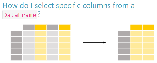
Selecting Columns
First things first. If we want to look the contents of a single column, we could do it like this, specifying the column name after the . without parentheses:
country_metrics.country0 Afghanistan
1 Afghanistan
2 Afghanistan
3 Afghanistan
4 Afghanistan
...
1699 Zimbabwe
1700 Zimbabwe
1701 Zimbabwe
1702 Zimbabwe
1703 Zimbabwe
Name: country, Length: 1704, dtype: objectWhen we want to select more than one column to include in our dataframe, we use the convention df[['col1', 'col2']] to select the columns we want.
In our example below, we will create a new dataframe called narrow_country_metrics. We are primarily interested in getting the population metric from the original dataset, and since we want to be able to analyze it by year, country, and continent, we will add those into our new dataframe also. So the dataset will be more narrow than the one it was created from.
There are two ways to approach this. The first way to approach is to identify all the columns you want to keep.
narrow_country_metrics = country_metrics[
    ['country', 'year', 'pop', 'continent']
    ]
narrow_country_metrics.head(2)| country | year | pop | continent | |
|---|---|---|---|---|
| 0 | Afghanistan | 1952 | 8425333.0 | Asia |
| 1 | Afghanistan | 1957 | 9240934.0 | Asia |
The second way is use the pandas .drop() method to eliminate the columns from the original object that you do not want to keep. Thus in the end we can achieve the same result as the example above by simply dropping two variables instead of naming four. With this method, we also need to add the specification axis = 1, which indicates that it is columns (and not rows) being referenced for being dropped.
narrow_country_metrics = country_metrics.drop(
    ['lifeExp', 'gdpPercap'], axis=1
    )
narrow_country_metrics.head(2)| country | year | pop | continent | |
|---|---|---|---|---|
| 0 | Afghanistan | 1952 | 8425333.0 | Asia |
| 1 | Afghanistan | 1957 | 9240934.0 | Asia |
Either way we have a more manageable dataset to work with called narrow_country_metrics. The original dataframe country_metrics is still there, and it still the same shape as before, we have not changed it.
However, it is important to realize that in python it is very common to change an object by referring to that object on both sides of the assignment operator. In the code below, we narrow the narrow_country_metrics dataset down even further by removing the column pop as well.
narrow_country_metrics = narrow_country_metrics.drop(['pop'], axis=1)
narrow_country_metrics.head(2)| country | year | continent | |
|---|---|---|---|
| 0 | Afghanistan | 1952 | Asia |
| 1 | Afghanistan | 1957 | Asia |
If we want to have the pop variable back in the narrow_country_metrics object, we will need to recreate it from the source it came from, where pop was still intact.
TipReminder on Assignment!
When you create a variable or dataframe object in python, to the left of the = sign you always put the name of the object you want to make or modify. To the right, that’s where you put the content that shows how the existing object is to be modified. It may feel counterintuitive but don’t be concerned, it is the standard way that the code is structured to be understood.
6.3 Selecting rows
Of course, in data analysis we are usually interested in looking at just some rows of data, not all rows all the time.
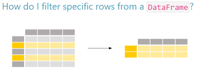
Selecting Rows
Relational operators
When we want to look at just selected rows (i.e. select rows that have certain values within a given column) we can supply a condition that must be met for a given row in that column. To do this, we must use one of the following comparison operators, which are also called relational operators:
- equal to
== - not equal to
!= - less than
< - greater than
> - less than or equal to
<= - greater than or equal to
>=
Let’s try an example. The most commonly used relational operator is likely equal to (==). In the example below we have a statement that pandas evaluates line by line in the dataframe as to whether it corresponds to a boolean value of True or False.
country_metrics['year'] == 19720 False
1 False
2 False
3 False
4 True
...
1699 False
1700 False
1701 False
1702 False
1703 False
Name: year, Length: 1704, dtype: boolWhen we create an object from this evaluation in pandas, it returns to that object only the rows that evaluate as True:
filtered_country_metrics = country_metrics[country_metrics['year'] == 1972]
filtered_country_metrics.head(2)| country | year | pop | continent | lifeExp | gdpPercap | |
|---|---|---|---|---|---|---|
| 4 | Afghanistan | 1972 | 13079460.0 | Asia | 36.088 | 739.981106 |
| 16 | Albania | 1972 | 2263554.0 | Europe | 67.690 | 3313.422188 |
Logical operators
In python, it is common to use the logical operators and, or, and not to evaluate expressions. For example, as in the code below, python evaluates the and to see whether BOTH operands are true:
x = 5
print(x > 3 and x < 10)TrueHowever, when we ask pandas to evaluate whether a set of logical relations exist within a pandas series object, we must use pandas bitwise logical operators, whose syntax is different:
- and
& - or
| - not
~
When combining multiple conditional statements in a pandas series object, each condition must be surrounded by parentheses () within the square brackets []. In the example below, we use an & to indicate that both conditions must be true for a row to be returned:
filtered_country_metrics = country_metrics[
    (country_metrics['year'] == 1972) &
    (country_metrics['country'] == 'Albania')
    ]
filtered_country_metrics.head()| country | year | pop | continent | lifeExp | gdpPercap | |
|---|---|---|---|---|---|---|
| 16 | Albania | 1972 | 2263554.0 | Europe | 67.69 | 3313.422188 |
In the example above, there is only one row of data that matches the condition.
We can use the | which indicates that if either or both of the conditions are true for a given row, that row is returned into the object:
filtered_country_metrics = country_metrics[
    (country_metrics['year'] == 1972) |
    (country_metrics['country'] == 'Albania')
    ]
filtered_country_metrics.head()| country | year | pop | continent | lifeExp | gdpPercap | |
|---|---|---|---|---|---|---|
| 4 | Afghanistan | 1972 | 13079460.0 | Asia | 36.088 | 739.981106 |
| 12 | Albania | 1952 | 1282697.0 | Europe | 55.230 | 1601.056136 |
| 13 | Albania | 1957 | 1476505.0 | Europe | 59.280 | 1942.284244 |
| 14 | Albania | 1962 | 1728137.0 | Europe | 64.820 | 2312.888958 |
| 15 | Albania | 1967 | 1984060.0 | Europe | 66.220 | 2760.196931 |
In the example above, there are many rows that satisfy one or the other condition. As an aside, were we to want to know how many rows fulfill this | situation, we could have called the .info() method instead of .head().
You will find that it is very common within python/pandas to see the .iloc() function used, so it is worthwhile to give that a brief introduction also.
This function enables the selection of data from a particular row or column, according to the integer based position index as shown in the image below:

Row and column values iloc() refers to
By referring to these locations, we can use iloc() to retrieve the exact cells we want to see. For example, if we just want the row of data corresponding to the index integer value 5, we would run the following code:
country_metrics.iloc[5]country Afghanistan
year 1977
pop 14880372.0
continent Asia
lifeExp 38.438
gdpPercap 786.11336
Name: 5, dtype: objectWe can also modify the above call to look at column(s)! For example, we specify the row(s) of interest to the left of a comma in the square brackets, and the column(s) of interest to the right of it. In the example below, the code will retrieve just the content found at the intersection of row 5 and column 3:
country_metrics.iloc[5,3]'Asia'We can also retrieve ranges of rows and columns respectively by employing a colon along with the starting and ending rows or columns we want. In the example below, we want to get rows “0” through “2” and the columns “0” through “3”:
country_metrics.iloc[0:2,0:3]| country | year | pop | |
|---|---|---|---|
| 0 | Afghanistan | 1952 | 8425333.0 |
| 1 | Afghanistan | 1957 | 9240934.0 |
It is a flexible tool that can be very helpful as you build and review your code.
6.4 Sorting rows
So now you’ve mastered how to select rows and columns you want, congratulations! Instead of hunting and pecking for insights, one way to quickly make some sense of the data is to sort it - something you probably do in Excel all the time.
Let’s say we wanted to know more about Asian countries since 2002. First we should go ahead and create a dataframe that consists of just the data we are wanting to look at.
countries_2000s = country_metrics[
    (country_metrics['year'] >= 2002) &
    (country_metrics['continent'] == 'Asia')
    ]
countries_2000s.head()| country | year | pop | continent | lifeExp | gdpPercap | |
|---|---|---|---|---|---|---|
| 10 | Afghanistan | 2002 | 25268405.0 | Asia | 42.129 | 726.734055 |
| 11 | Afghanistan | 2007 | 31889923.0 | Asia | 43.828 | 974.580338 |
| 94 | Bahrain | 2002 | 656397.0 | Asia | 74.795 | 23403.559270 |
| 95 | Bahrain | 2007 | 708573.0 | Asia | 75.635 | 29796.048340 |
| 106 | Bangladesh | 2002 | 135656790.0 | Asia | 62.013 | 1136.390430 |
This is a nice start. But to see some meaningful insights it is helpful to sort the metric we are interested in something other than the default way the data appear positioned in the dataframe.
The .sort_values() method let’s us specify a column (or multiple columns) we want to sort and enter an argument that indicates in which direction we would like it to be sorted, from low to high or vice-versa. We want life expectancy from high to low, so the ascending parameter should be set to False.
countries_2000s = countries_2000s.sort_values('lifeExp', ascending=False)
countries_2000s.head()| country | year | pop | continent | lifeExp | gdpPercap | |
|---|---|---|---|---|---|---|
| 803 | Japan | 2007 | 127467972.0 | Asia | 82.603 | 31656.06806 |
| 671 | Hong Kong China | 2007 | 6980412.0 | Asia | 82.208 | 39724.97867 |
| 802 | Japan | 2002 | 127065841.0 | Asia | 82.000 | 28604.59190 |
| 670 | Hong Kong China | 2002 | 6762476.0 | Asia | 81.495 | 30209.01516 |
| 767 | Israel | 2007 | 6426679.0 | Asia | 80.745 | 25523.27710 |
That was pretty straightforward and it helps us get more insights. Looks like Japan, in 2007, was the Asian country with the highest life expectancy.
Often one will want to sort by more than one column. To do that, instead of passing in a single column, we pass in a list of the columns we want to sort on. We can also control whether we would like each column to be sorted in ascending or descending order by passing in a respective list of boolean values in the ascending= parameter. In the example below, the code indicates that we want to sort first by ‘country’ in reverse alphabetical order, then by life expectancy from high to low.
countries_2000s = countries_2000s.sort_values(
    ['country', 'lifeExp'], ascending=[False, False]
    )
countries_2000s.head()| country | year | pop | continent | lifeExp | gdpPercap | |
|---|---|---|---|---|---|---|
| 1679 | Yemen Rep. | 2007 | 22211743.0 | Asia | 62.698 | 2280.769906 |
| 1678 | Yemen Rep. | 2002 | 18701257.0 | Asia | 60.308 | 2234.820827 |
| 1667 | West Bank and Gaza | 2007 | 4018332.0 | Asia | 73.422 | 3025.349798 |
| 1666 | West Bank and Gaza | 2002 | 3389578.0 | Asia | 72.370 | 4515.487575 |
| 1655 | Vietnam | 2007 | 85262356.0 | Asia | 74.249 | 2441.576404 |
We see that when we created and sorted this new object, the index values are those that were associated with the original country_metrics dataframe.
Depending on what we want to do with countries_2000s going forward, we might want to create a new “default” index for it instead of the existing one. That’s where the .reset_index() function comes into play.
In the code below, we reset the index.
countries_2000s = countries_2000s.reset_index(drop=False)
countries_2000s.head()| index | country | year | pop | continent | lifeExp | gdpPercap | |
|---|---|---|---|---|---|---|---|
| 0 | 1679 | Yemen Rep. | 2007 | 22211743.0 | Asia | 62.698 | 2280.769906 |
| 1 | 1678 | Yemen Rep. | 2002 | 18701257.0 | Asia | 60.308 | 2234.820827 |
| 2 | 1667 | West Bank and Gaza | 2007 | 4018332.0 | Asia | 73.422 | 3025.349798 |
| 3 | 1666 | West Bank and Gaza | 2002 | 3389578.0 | Asia | 72.370 | 4515.487575 |
| 4 | 1655 | Vietnam | 2007 | 85262356.0 | Asia | 74.249 | 2441.576404 |
Notice how the original index now is turned into a column itself called “index”. Depending on the use case, we might want to keep this column in the new dataframe. For example, if we ultimately wanted to join this dataframe back with the original it could act as a key. If we know, however, that it is of no value anymore to us, we can and probably should delete it. To do this, we would have set the drop parameter above to True.
Let’s use the iloc() method to look at the positional content of this countries_2000s object and confirm that Yeman shows up in row 0 as we expect.
countries_2000s.iloc[0:4,0:5]| index | country | year | pop | continent | |
|---|---|---|---|---|---|
| 0 | 1679 | Yemen Rep. | 2007 | 22211743.0 | Asia |
| 1 | 1678 | Yemen Rep. | 2002 | 18701257.0 | Asia |
| 2 | 1667 | West Bank and Gaza | 2007 | 4018332.0 | Asia |
| 3 | 1666 | West Bank and Gaza | 2002 | 3389578.0 | Asia |
6.5 Putting multiple methods together
The next step is usually to bring several of these commands together to get a nicely refined look at the data. Essentially you will need to invoke a number of calls sequentially to some object, with each one in turn performing some action on it.
A common approach is to put the object name on each sucessive line of code along with the = operator as well as the modifying code to the right. Imagine we were given the following task:
- Select only the rows where the country is equal to Ireland AND where the year is 1992 or greater
- Take these rows and sort them by year, going from high to low values, top to bottom
The example below shows how we would employ the line-by-line approach:
chained2_df = country_metrics[(country_metrics['country'] == 'Ireland')]
chained2_df = chained2_df[(chained2_df['year'] >= 1992)]
chained2_df = chained2_df.sort_values('year', ascending=False)
chained2_df.head(3)| country | year | pop | continent | lifeExp | gdpPercap | |
|---|---|---|---|---|---|---|
| 755 | Ireland | 2007 | 4109086.0 | Europe | 78.885 | 40675.99635 |
| 754 | Ireland | 2002 | 3879155.0 | Europe | 77.783 | 34077.04939 |
| 753 | Ireland | 1997 | 3667233.0 | Europe | 76.122 | 24521.94713 |
You can read fairly clearly what is happening in each line.
You can also put multiple methods in the same line of code, as long as you separate each of the elements. In pandas, this is sometimes referred to as joining or chaining, as you are essentially creating a joining/chaining actions together.
The code below accomplishes what the more verbose code above does but in a more efficient way:
chained_df = country_metrics[
    (country_metrics['country'] == 'Ireland') &
    (country_metrics['year'] >= 1992)
    ].sort_values('year', ascending = False)
chained_df.head(3)| country | year | pop | continent | lifeExp | gdpPercap | |
|---|---|---|---|---|---|---|
| 755 | Ireland | 2007 | 4109086.0 | Europe | 78.885 | 40675.99635 |
| 754 | Ireland | 2002 | 3879155.0 | Europe | 77.783 | 34077.04939 |
| 753 | Ireland | 1997 | 3667233.0 | Europe | 76.122 | 24521.94713 |
Each line is executed in sequence, so be careful when constructing code that the order in which you modify your dataframe is what you intend. Take the example below, in which we want to find European values for GDP per capita. In it, we first have a line of code that selects the rows that contain “Europe” in the first line, then looks at the column values for “year”, “country”, and “gdpPercap”.
year_country_gdp = country_metrics[
    (country_metrics['continent'] == 'Europe')
    ]
year_country_gdp = year_country_gdp[['year', 'country', 'gdpPercap']]
year_country_gdp.head(3)| year | country | gdpPercap | |
|---|---|---|---|
| 12 | 1952 | Albania | 1601.056136 |
| 13 | 1957 | Albania | 1942.284244 |
| 14 | 1962 | Albania | 2312.888958 |
Had we reversed the lines of code, and selected the “year”, “country”, and “gdpPercap” columns first to put into our new object, we would not have been able to sort for “Europe” in the “continent” column, as the “continent” would have been essentially removed from the dataframe in the step above. So an error would have been thrown.
6.6 Creating new columns of data
Very often we have some data in our dataset that we want to transform to give us additional information. In Excel this is something that is done all the time by creating a formula in a cell that refers to other columns and applies some sort of logic or mathematical expression to it.
There are different ways you can go about this in pandas. The most straightforward way is to define a new column on the left of the = and then reference the existing column and whatever additional conditions you would like on the right. In the example below, the existing population variable “pop” is converted to a value that shows population in millions.
new_cols_df = country_metrics
new_cols_df['pop_millions'] = new_cols_df['pop']/1000000
new_cols_df.head(2)| country | year | pop | continent | lifeExp | gdpPercap | pop_millions | |
|---|---|---|---|---|---|---|---|
| 0 | Afghanistan | 1952 | 8425333.0 | Asia | 28.801 | 779.445314 | 8.425333 |
| 1 | Afghanistan | 1957 | 9240934.0 | Asia | 30.332 | 820.853030 | 9.240934 |
Another way is to call the pandas function apply() in which other, more complicated functions can be passed for a given column. This could be a complicated mathematical formula, a function acting on strings or dates, or any other function that cannot be represented by a simple multiplication or division. In the example below, the len() function is applied to each row in the “country” column and a new column with the number of characters for that row is returned:
new_cols_df['country_name_chars'] = new_cols_df.country.apply(len)
new_cols_df.sample(5)| country | year | pop | continent | lifeExp | gdpPercap | pop_millions | country_name_chars | |
|---|---|---|---|---|---|---|---|---|
| 755 | Ireland | 2007 | 4109086.0 | Europe | 78.885 | 40675.996350 | 4.109086 | 7 |
| 904 | Libya | 1972 | 2183877.0 | Africa | 52.773 | 21011.497210 | 2.183877 | 5 |
| 819 | Kenya | 1967 | 10191512.0 | Africa | 50.654 | 1056.736457 | 10.191512 | 5 |
| 587 | Ghana | 2007 | 22873338.0 | Africa | 60.022 | 1327.608910 | 22.873338 | 5 |
| 1464 | Sweden | 1952 | 7124673.0 | Europe | 71.860 | 8527.844662 | 7.124673 | 6 |
There is also a special python function called lambda. It is known as an anonymous function, appears in a single line of code, and is not given a name other than lambda. It can take any number of arguments in an expression.
The .assign() method looks at this expression with lambda in it and returns the value it is asked to do and assigns it to the variable name given it. This is how it comes all together to give us actual GDP for each row in our dataframe:
GDP_df = new_cols_df.assign(GDP=lambda x: x['pop'] * x['gdpPercap'])
GDP_df.head(5)| country | year | pop | continent | lifeExp | gdpPercap | pop_millions | country_name_chars | GDP | |
|---|---|---|---|---|---|---|---|---|---|
| 0 | Afghanistan | 1952 | 8425333.0 | Asia | 28.801 | 779.445314 | 8.425333 | 11 | 6.567086e+09 |
| 1 | Afghanistan | 1957 | 9240934.0 | Asia | 30.332 | 820.853030 | 9.240934 | 11 | 7.585449e+09 |
| 2 | Afghanistan | 1962 | 10267083.0 | Asia | 31.997 | 853.100710 | 10.267083 | 11 | 8.758856e+09 |
| 3 | Afghanistan | 1967 | 11537966.0 | Asia | 34.020 | 836.197138 | 11.537966 | 11 | 9.648014e+09 |
| 4 | Afghanistan | 1972 | 13079460.0 | Asia | 36.088 | 739.981106 | 13.079460 | 11 | 9.678553e+09 |
So now we can see the newly created column “GDP” and see the value for each country in our new object. Notice that the GDP data is in scientific notation (i.e. the decimal number times x number of zeros), so it’s a bit hard to read. If we wanted readers to consume that data we would go ahead and change the data type for it. But for current purposes we’ll leave that alone.
6.7 Joining datasets together
One of the most important tasks in data analysis is to be able to join multiple datasets together. With pandas, there are functions called .merge() and .join() that are similar to each other. As .merge() is perhaps the more used, intuitive, and powerful of the two, we will introduce that method in this tutorial in some depth. There is also a cool function called .concat() that will be introduced below as well.
But first, let’s get a second file that gives us country size in square kilometers by country. We will use this data to put together with our country_metrics dataframe.
country_size_url = "https://raw.githubusercontent.com/bcgov/"\
    "ds-intro-to-python/main/data/countrysize.csv"
country_size = pd.read_csv(country_size_url, encoding= 'unicode_escape')
country_size.info()
country_size.sample(2)
<class 'pandas.core.frame.DataFrame'>
RangeIndex: 235 entries, 0 to 234
Data columns (total 2 columns):
# Column Non-Null Count Dtype
--- ------ -------------- -----
0 nation 235 non-null object
1 area_square_kms 235 non-null int64
dtypes: int64(1), object(1)
memory usage: 3.8+ KB| nation | area_square_kms | |
|---|---|---|
| 133 | Netherlands | 41850 |
| 104 | Bulgaria | 110879 |
Ok, this country_size dataset looks like we expect - a list of countries alongside the land size of that country in square kilometers. There are some omissions in this list - not all countries in our country_metrics dataset are present in this country_size object. But for our present purposes this is ok. We just want to get that square kilometers data into a combined dataset and it is sufficient for that.
Essentially what we want to do is a classic “left-join” operation of the sort in the diagram below. Conceptually, the country_metrics dataset is like the purple table and the country_size dataset is like the red one.
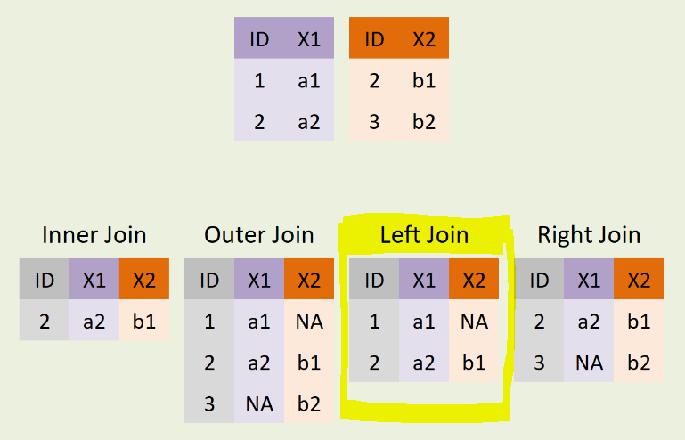
Types of Joins
The .merge() method (with reference material available here) works similarly to how table joining works in SQL or how the VLOOKUP function works in Excel. One needs to specify both dataframes, the key variables on which to join them, and the kind of join desired.
So let’s look at the example below to see how it all comes together in code.
combined_df = country_metrics.merge(
    country_size,
    left_on='country',
    right_on='nation',
    how='left'
    )
combined_df.head(2)| country | year | pop | continent | lifeExp | gdpPercap | pop_millions | country_name_chars | nation | area_square_kms | |
|---|---|---|---|---|---|---|---|---|---|---|
| 0 | Afghanistan | 1952 | 8425333.0 | Asia | 28.801 | 779.445314 | 8.425333 | 11 | Afghanistan | 652230.0 |
| 1 | Afghanistan | 1957 | 9240934.0 | Asia | 30.332 | 820.853030 | 9.240934 | 11 | Afghanistan | 652230.0 |
When you run the code above you will notice that both the nation key column and the area_square_kms column have been joined together in the new combined_df object. One can keep that nation column in there for control purposes, or it can be removed by using the .drop() method we used earlier:
combined_df = combined_df.drop('nation', axis=1)
combined_df.head()| country | year | pop | continent | lifeExp | gdpPercap | pop_millions | country_name_chars | area_square_kms | |
|---|---|---|---|---|---|---|---|---|---|
| 0 | Afghanistan | 1952 | 8425333.0 | Asia | 28.801 | 779.445314 | 8.425333 | 11 | 652230.0 |
| 1 | Afghanistan | 1957 | 9240934.0 | Asia | 30.332 | 820.853030 | 9.240934 | 11 | 652230.0 |
| 2 | Afghanistan | 1962 | 10267083.0 | Asia | 31.997 | 853.100710 | 10.267083 | 11 | 652230.0 |
| 3 | Afghanistan | 1967 | 11537966.0 | Asia | 34.020 | 836.197138 | 11.537966 | 11 | 652230.0 |
| 4 | Afghanistan | 1972 | 13079460.0 | Asia | 36.088 | 739.981106 | 13.079460 | 11 | 652230.0 |
Another innovative way to put “merge” data together in pandas is with the .concat() function. Conceptually you can think if it like “stacking” two data objects on top of each other or side-by-side as shown in the diagram below.
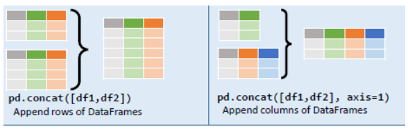
Ways to stack data
To illustrate, let’s fetch two simple dataframes. Each contains the average scores for three subjects by year for two separate schools.
school1_url  = "https://raw.githubusercontent.com/bcgov/"\
    "ds-intro-to-python/main/data/school1.csv"
school2_url  = "https://raw.githubusercontent.com/bcgov/"\
    "ds-intro-to-python/main/data/school2.csv"
school1_df = pd.read_csv(school1_url)
school2_df = pd.read_csv(school2_url)
Let’s take a quick look at the two dataframes.
school1_df| Subject | Avg Score 2018 | Avg Score 2019 | Avg Score 2020 | |
|---|---|---|---|---|
| 0 | Science | 67 | 88 | 89 |
| 1 | English | 86 | 67 | 77 |
| 2 | Math | 84 | 73 | 75 |
school2_df| Subject | Avg Score 2018 | Avg Score 2019 | Avg Score 2020 | |
|---|---|---|---|---|
| 0 | Science | 32 | 88 | 90 |
| 1 | English | 88 | 44 | 77 |
| 2 | Math | 84 | 73 | 53 |
We call .concat() and pass in the objects that we want to stack vertically. This is a similiar operation to union in SQL.
vertical_stack_df = pd.concat([school1_df, school2_df])
vertical_stack_df| Subject | Avg Score 2018 | Avg Score 2019 | Avg Score 2020 | |
|---|---|---|---|---|
| 0 | Science | 67 | 88 | 89 |
| 1 | English | 86 | 67 | 77 |
| 2 | Math | 84 | 73 | 75 |
| 0 | Science | 32 | 88 | 90 |
| 1 | English | 88 | 44 | 77 |
| 2 | Math | 84 | 73 | 53 |
It is also possible to stack the data horizontally. Here it is necessary to specify the columnar axis (axis=1) as the default setting is for rows (axis=0).
horizontal_stack = pd.concat([school1_df, school2_df], axis=1)
horizontal_stack| Subject | Avg Score 2018 | Avg Score 2019 | Avg Score 2020 | Subject | Avg Score 2018 | Avg Score 2019 | Avg Score 2020 | |
|---|---|---|---|---|---|---|---|---|
| 0 | Science | 67 | 88 | 89 | Science | 32 | 88 | 90 |
| 1 | English | 86 | 67 | 77 | English | 88 | 44 | 77 |
| 2 | Math | 84 | 73 | 75 | Math | 84 | 73 | 53 |
This introduction only scratches the surface of how to leverage this way of joining datasets together. But it can be a powerful tool in the toolkit for the right use case. More detail found here.
6.8 Grouping and summarizing
Sometimes of course one would prefer to group rows together for the purpose of summarizing them in various ways.
In pandas, we can accomplish this using the .groupby() method. A .groupby() operation involves some combination of splitting the object, applying a function, and combining the results. It is used together with one or more aggregation functions:
count(): Total number of itemsfirst(),last(): First and last itemmean(),median(): Mean and medianmin(),max(): Minimum and maximumstd(),var(): Standard deviation and variancemad(): Mean absolute deviationprod(): Product of all itemssum(): Sum of all items
First let us look at a simple example where we want to get the mean life expectancy for each continent in the data. To do this, we would use the groupby() function to call the appropriate segment (i.e. continent), metric (i.e. lifeExp), and type of aggregation (i.e. mean):
simple_mean = country_metrics.groupby('continent').lifeExp.mean()
simple_mean
continent
Africa 48.865330
Americas 64.658737
Asia 60.064903
Europe 71.903686
Oceania 74.326208
Name: lifeExp, dtype: float64Fortunately, if we want to look at several aggregations at once, we can do that too. To extend our example above, we would specify the “continent” column in the .groupby() function, then pass additional aggregation functions (in our case, we will add “mean”, “min”, and “max”) as a dictionary within the .agg() function.
TipRecall: Dictionaries in Python
Remember that a dictionary in Python language is a particular type of data structure that contains a collection of key: value pairs. It is analogous to a regular word dictionary you are familiar with which is a collection of words to their meanings. Python dictionaries allow us to associate a value to a unique key, and then to quickly access this value. They are generally created within curly braces {} and have a specified key name and value (e.g. basic form for a python dictionary {"key1": "value1"})
This dictionary takes the column that we are aggregating - in this case life expectancy - as a key and a list of aggregation functions as its value. We also add a line of code that gives each of the columns a new name with the .columns() function.
grouped_single = country_metrics.groupby('continent') \
    .agg({'lifeExp': ['mean', 'min', 'max']})
grouped_single.columns = ['lifeExp_mean', 'lifeExp_min', 'lifeExp_max']
grouped_single| lifeExp_mean | lifeExp_min | lifeExp_max | |
|---|---|---|---|
| continent | |||
| Africa | 48.865330 | 23.599 | 76.442 |
| Americas | 64.658737 | 37.579 | 80.653 |
| Asia | 60.064903 | 28.801 | 82.603 |
| Europe | 71.903686 | 43.585 | 81.757 |
| Oceania | 74.326208 | 69.120 | 81.235 |
If you look closely at grouped_single you see that the variable “continent” is on a different line than are the columns that are aggregated. That is because continent in this instance is actually an index and not a column.
We can nest additional “groups within groups” by creating a list of column names and passing them to the .groupby() function instead of passing a single value.
The example below adds more granularity with the introduction of ‘country’ and the creation of a list to hold both ‘continent’ and ‘country’.
grouped_multiple = country_metrics.groupby(
    ['continent', 'country']).agg({'pop': ['mean', 'min', 'max']}
    )
grouped_multiple.columns = ['pop_mean', 'pop_min', 'pop_max']
grouped_multiple.head(10)| pop_mean | pop_min | pop_max | ||
|---|---|---|---|---|
| continent | country | |||
| Africa | Algeria | 1.987541e+07 | 9279525.0 | 33333216.0 |
| Angola | 7.309390e+06 | 4232095.0 | 12420476.0 | |
| Benin | 4.017497e+06 | 1738315.0 | 8078314.0 | |
| Botswana | 9.711862e+05 | 442308.0 | 1639131.0 | |
| Burkina Faso | 7.548677e+06 | 4469979.0 | 14326203.0 | |
| Burundi | 4.651608e+06 | 2445618.0 | 8390505.0 | |
| Cameroon | 9.816648e+06 | 5009067.0 | 17696293.0 | |
| Central African Republic | 2.560963e+06 | 1291695.0 | 4369038.0 | |
| Chad | 5.329256e+06 | 2682462.0 | 10238807.0 | |
| Comoros | 3.616839e+05 | 153936.0 | 710960.0 |
Again will notice that this dataframe looks a little different than some others we have seen in that there are blank spaces below each grouped value of continent in that index. This object is a multi-indexed dataframe. It presents the data nicely to consume visually, but it is not ideal to work with if you want to do further manipulation.
This is likely again a good time to use the reset_index() function. This is a step that resets the index to an integer based index and re-creates a non-indexed pandas dataframe.
The code block below is identical to the one we just ran except for the line of code that resets the index:
grouped_multiple = country_metrics.groupby(
    ['continent', 'country']).agg({'pop': ['mean', 'min', 'max']}
    )
grouped_multiple.columns = ['pop_mean', 'pop_min', 'pop_max']
grouped_multiple = grouped_multiple.reset_index()  # resets the index
grouped_multiple.head(10)| continent | country | pop_mean | pop_min | pop_max | |
|---|---|---|---|---|---|
| 0 | Africa | Algeria | 1.987541e+07 | 9279525.0 | 33333216.0 |
| 1 | Africa | Angola | 7.309390e+06 | 4232095.0 | 12420476.0 |
| 2 | Africa | Benin | 4.017497e+06 | 1738315.0 | 8078314.0 |
| 3 | Africa | Botswana | 9.711862e+05 | 442308.0 | 1639131.0 |
| 4 | Africa | Burkina Faso | 7.548677e+06 | 4469979.0 | 14326203.0 |
| 5 | Africa | Burundi | 4.651608e+06 | 2445618.0 | 8390505.0 |
| 6 | Africa | Cameroon | 9.816648e+06 | 5009067.0 | 17696293.0 |
| 7 | Africa | Central African Republic | 2.560963e+06 | 1291695.0 | 4369038.0 |
| 8 | Africa | Chad | 5.329256e+06 | 2682462.0 | 10238807.0 |
| 9 | Africa | Comoros | 3.616839e+05 | 153936.0 | 710960.0 |
This looks more like the structure of the dataframes we know already and will be easier to manipulate further.
By now you should be able to select the rows and columns, join together dataframes, and create some basic summarizations of data. The next section will look at some of the more sophisticated and elegant tools for understanding and presenting your data. But the building blocks you have just learned about are the meat and potatoes of data analysis in the python world.