This report is to document the sensitivity of the TUV model, and the subsequent calculation of water quality guidelines for *PACs, to variation in certain TUV parameters.
*Note that in some places in the code, the term
pah(polycyclic aromatic hydrocarbons) is used in place ofpac(polycyclic aromatic compounds).
Input parameters
The input parameters for the calculation of light attenuation through water for the TUV model are:
- Vertical Attenuation Coefficient at wavelength
wvl:-
KdLight attenuation coefficient (set directly or calculated from DOC) -
Sk(default0.018) -
ref_wvlReference wavelength forKd(default305)
-
-
depth_mWater depth in m -
latLatitude in decimal degrees -
lonLongitude in decimal degrees -
elev_mSurface elevation, m above sea level -
yearYear -
monthMonth -
dayDay -
tzoneTimezone Local Time - UTC (default0; UTC) -
tstartStart time, hours local time (default0) -
tstopStop time, hours local time (default23) -
tstepsNumber of time steps (default24) -
albedoSurface albedo (default0.07) -
o3_tcOzone column, Dobson Units (DU) - Looked up in climatology (recommended default300) -
so2_tcSO2 column, DU (default0) -
no2_tcNO2 column, DU (default0) -
taucldCloud optical depth (default0) -
zbaseCloud base, km (default4) -
ztopCloud top, km (default5) -
tauaerAerosol optical depth at 550 nm - Looked up in climatology (recommended default0.235) -
ssaaerAerosol single scattering albedo (default0.990) -
alphaAerosol Angstrom exponent(default1.0) -
wvl_startStarting wavelength, nm (default279.5) -
wvl_endEnd wavelength, nm (default420.5) -
wvl_stepsNumber of wavelength intervals (default141) -
nstrTUV run type; use -2 for fast, 4 for slightly more accurate (default-2)
Those currently under consideration for sensitivity analysis are:
-
KdLight attenuation coefficient - includes use ofDOCfor calculatingKd -
albedoSurface albedo (default0.07) -
o3_tcOzone column, Dobson Units (DU) - Looked up in climatology (recommended default300) -
tauaerAerosol optical depth at 550 nm - Looked up in climatology (recommended default0.235) -
ssaaerAerosol single scattering albedo (default0.990) -
latLatitude in decimal degrees -
elev_mSurface elevation, m above sea level -
depth_mWater depth in m -
nstrTUV run type; use -2 for fast, 4 for slightly more accurate (default-2)
The analyses are conducted at three different sample lakes (Southern Interior, Vancouver Island, Northeast), using two PACs (Anthracene and Benzo[a]pyrene).
For each analysis, we will test a range of reasonable values for the parameter of interest, and plot the phototoxic benchmark value calculated across that range. To look at the relative effect of that parameter on the photoxicity of the PAC, we also plot the ratio of phototoxic:narcotic benchmark.
Initially, sensitivity analyses will be univariate (varying the input of interest while holding the others constant). If there are significant interactions expected between certain variables, these can be explored.
Basic usage of the pahwq package
To start, we will demonstrate a typical straightforward use case at a single site.
To calculate the acute phototoxic water quality guideline (phototoxic benchmark) for Anthracene at 0.25 m depth in Okanagan Lake on June 21, 2023, with a measured DOC of 5 g/m^3, you would use the following code:
First, set up the options for the model run:
library(pahwq)

set_tuv_aq_params(
  depth_m = 0.25,
  lat = 49.601632,
  lon = -119.605862,
  elev_m = 342,
  DOC = 5,
  date = "2023-06-21",
  tzone = -8,
  albedo = 0.05
)
After setting them, you can view the options that will be used by
TUV. Some are set via the function inputs, some are looked up (e.g.,
o3_tc, tauaer) or calculated (e.g.,
kd(305) is calculated from the input DOC).
view_tuv_aq_params()
#> a,b,c for: kvdom = a exp(-b(wvl-c)). a = kd(305), b = Sk, c = wavelength, wvl = 305: 10.67 0.018 305
#> ydepth, m: 0.25
#> lat, negative S of Equator: 49.601632
#> lon, negative W of Greenwich (zero) meridian: -119.605862
#> surface elevation, km above sea level: 0.342
#> timezone: Local Time - UTC: -8
#> iyear: 2023
#> imonth: 6
#> iday: 21
#> tstart, hours local time: 0
#> tstop, hours local time: 23
#> number of time steps: 24
#> surface albedo: 0.05
#> o3_tc  ozone column, Dobson Units (DU): 359.937
#> so2_tc SO2 column, DU: 0
#> no2_tc NO2 column, DU: 0
#> taucld - cloud optical depth: 0
#> zbase - cloud base, km: 4
#> ztop - cloud top, km: 5
#> tauaer - aerosol optical depth at 550 nm: 0.0641989811085006
#> ssaaer - aerosol single scattering albedo: 0.99
#> alpha - aerosol Angstrom exponent: 1
#> starting wavelength, nm: 279.5
#> end wavelength, nm: 800.5
#> number of wavelength intervals: 521
#> nstr, use -2 for fast, 4 for slightly more accurate: -2
#> out_irrad_y, T/F, planar spectral irradiance at ydepth: T
#> out_aflux_y, T/F, scalar spectral irradiance (actinic flux)  at depth: F
#> out_irrad_ave, T/F, planar irrad., averaged 0-ydepth: F
#> out_aflux_ave, T/F, scalar, ave 0-ydepth: F
#> out_irrad_atm, T/F, planar, in atmosphere: F
#> out_aflux_atm, T/F, scalar, in atmosphere: F
Run the TUV model and get the results. The results show the underwater irradiance at the specified depth, at each wavelength and time step.
run_tuv()

# Get the results
tuv_res <- get_tuv_results(file = "out_irrad_y")
head(tuv_res)
#>    wl wavelength_start wavelength_end Kd_lambda t_00.00.00 t_01.00.00
#> 1 280            279.5          280.5      16.7          0          0
#> 2 281            280.5          281.5      16.4          0          0
#> 3 282            281.5          282.5      16.1          0          0
#> 4 283            282.5          283.5      15.9          0          0
#> 5 284            283.5          284.5      15.6          0          0
#> 6 285            284.5          285.5      15.3          0          0
#>   t_02.00.00 t_03.00.00 t_04.00.00 t_05.00.00 t_06.00.00 t_07.00.00 t_08.00.00
#> 1          0          0   1.93e-36   6.12e-36   1.16e-35   2.71e-35   5.35e-32
#> 2          0          0   1.83e-33   5.79e-33   1.10e-32   2.63e-32   3.85e-29
#> 3          0          0   1.99e-30   6.28e-30   1.21e-29   2.96e-29   3.14e-26
#> 4          0          0   9.11e-29   2.88e-28   5.56e-28   1.39e-27   1.23e-24
#> 5          0          0   1.02e-26   3.22e-26   6.27e-26   1.61e-25   1.10e-22
#> 6          0          0   7.61e-25   2.40e-24   4.73e-24   1.26e-23   6.49e-21
#>   t_09.00.00 t_10.00.00 t_11.00.00 t_12.00.00 t_13.00.00 t_14.00.00 t_15.00.00
#> 1   2.39e-27   1.32e-24   3.76e-23   1.08e-22   3.82e-23   1.37e-24   2.56e-27
#> 2   6.55e-25   2.07e-22   4.39e-21   1.15e-20   4.46e-21   2.14e-22   6.97e-25
#> 3   1.99e-22   3.56e-20   5.61e-19   1.34e-18   5.69e-19   3.67e-20   2.11e-22
#> 4   4.43e-21   5.70e-19   7.57e-18   1.72e-17   7.68e-18   5.88e-19   4.67e-21
#> 5   1.88e-19   1.57e-17   1.66e-16   3.49e-16   1.68e-16   1.61e-17   1.97e-19
#> 6   5.11e-18   2.72e-16   2.27e-15   4.45e-15   2.30e-15   2.79e-16   5.34e-18
#>   t_16.00.00 t_17.00.00 t_18.00.00 t_19.00.00 t_20.00.00 t_21.00.00 t_22.00.00
#> 1   6.00e-32   2.74e-35   1.16e-35   6.16e-36   1.96e-36          0          0
#> 2   4.27e-29   2.66e-32   1.11e-32   5.82e-33   1.86e-33          0          0
#> 3   3.45e-26   2.99e-29   1.21e-29   6.32e-30   2.02e-30          0          0
#> 4   1.34e-24   1.40e-27   5.59e-28   2.90e-28   9.27e-29          0          0
#> 5   1.19e-22   1.63e-25   6.30e-26   3.24e-26   1.04e-26          0          0
#> 6   6.96e-21   1.28e-23   4.76e-24   2.42e-24   7.74e-25          0          0
#>   t_23.00.00
#> 1          0
#> 2          0
#> 3          0
#> 4          0
#> 5          0
#> 6          0
We can inspect and verify the inputs that were used in the model run:
tuv_run_params(tuv_res)
#> a,b,c for: kvdom = a exp(-b(wvl-c)). a = kd(305), b = Sk, c = wavelength, wvl = 305
#>                                                                   "10.67 0.018 305"
#>                                                                           ydepth, m
#>                                                                              "0.25"
#>                                                          lat, negative S of Equator
#>                                                                         "49.601632"
#>                                        lon, negative W of Greenwich (zero) meridian
#>                                                                       "-119.605862"
#>                                               surface elevation, km above sea level
#>                                                                             "0.342"
#>                                                          timezone: Local Time - UTC
#>                                                                                "-8"
#>                                                                               iyear
#>                                                                              "2023"
#>                                                                              imonth
#>                                                                                 "6"
#>                                                                                iday
#>                                                                                "21"
#>                                                            tstart, hours local time
#>                                                                                 "0"
#>                                                             tstop, hours local time
#>                                                                                "23"
#>                                                                number of time steps
#>                                                                                "24"
#>                                                                      surface albedo
#>                                                                              "0.05"
#>                                              o3_tc  ozone column, Dobson Units (DU)
#>                                                                           "359.937"
#>                                                               so2_tc SO2 column, DU
#>                                                                                 "0"
#>                                                               no2_tc NO2 column, DU
#>                                                                                 "0"
#>                                                        taucld - cloud optical depth
#>                                                                                 "0"
#>                                                              zbase - cloud base, km
#>                                                                                 "4"
#>                                                                ztop - cloud top, km
#>                                                                                 "5"
#>                                            tauaer - aerosol optical depth at 550 nm
#>                                                                "0.0641989811085006"
#>                                           ssaaer - aerosol single scattering albedo
#>                                                                              "0.99"
#>                                                   alpha - aerosol Angstrom exponent
#>                                                                                 "1"
#>                                                             starting wavelength, nm
#>                                                                             "279.5"
#>                                                                  end wavelength, nm
#>                                                                             "800.5"
#>                                                      number of wavelength intervals
#>                                                                               "521"
#>                                 nstr, use -2 for fast, 4 for slightly more accurate
#>                                                                                "-2"
#>                              out_irrad_y, T/F, planar spectral irradiance at ydepth
#>                                                                                 "T"
#>               out_aflux_y, T/F, scalar spectral irradiance (actinic flux)  at depth
#>                                                                                 "F"
#>                                out_irrad_ave, T/F, planar irrad., averaged 0-ydepth
#>                                                                                 "F"
#>                                            out_aflux_ave, T/F, scalar, ave 0-ydepth
#>                                                                                 "F"
#>                                           out_irrad_atm, T/F, planar, in atmosphere
#>                                                                                 "F"
#>                                           out_aflux_atm, T/F, scalar, in atmosphere
#>                                                                                 "F"
Next, calculate the site-specific light absorption
()
for Anthracene from the TUV results. The p_abs() function
uses a lookup table to get the molar absorption coefficient table for
the specified PAC.
(Pabs <- p_abs(tuv_res, "Anthracene"))
#> [1] 1135.67
Finally, calculate phototoxic benchmark in 𝝁g/L, supplying the value.
phototoxic_benchmark(Pabs, pah = "Anthracene")
#> [1] 2.151449
We can compare the phototoxic benchmark to the narcotic benchmark to see the effect of the photoxicity of the PAC:
narcotic_benchmark("Anthracene")
#> [1] 64.12872
A shortcut:
If you don’t need to inspect every step of the way, the above process can be completed in two function calls:
tuv_res <- tuv(
  depth_m = 0.25,
  lat = 49.601632,
  lon = -119.605862,
  elev_m = 342,
  DOC = 5,
  date = "2023-06-21",
  tzone = -8,
  albedo = 0.05
)

phototoxic_benchmark(tuv_res, "Anthracene")
#> [1] 2.151449
Sensitivity Analysis: Setup
We’ll start by loading the packages we need and getting some data from B.C. EMS:
Show/Hide Code
library(sf)
library(mapview)
library(rems)
library(dplyr)
library(ggplot2)
library(ggrepel)

con <- connect_historic_db()
db <- attach_historic_data(con)
sites_sf <- db |>
  filter(
    EMS_ID %in% c("0500236", "E207466", "0400390"),
    # grepl("(CHARLIE L)|(OKANAGAN)|(QUAMICHAN)", MONITORING_LOCATION),
    COLLECTION_START > as.Date("2020-01-01"),
    PARAMETER_CODE == "1103"
  ) |>
  collect() |>
  st_as_sf(coords = c("LONGITUDE", "LATITUDE"), crs = 4326, remove = FALSE) |>
  filter(!is.na(RESULT)) |>
  arrange(desc(COLLECTION_START)) |>
  group_by(EMS_ID, MONITORING_LOCATION, LONGITUDE, LATITUDE) |>
  mutate(doc_min = min(RESULT), doc_max = max(RESULT)) |>
  slice(1) |>
  select(
    emsid = EMS_ID,
    name = MONITORING_LOCATION,
    lon = LONGITUDE,
    lat = LATITUDE,
    date = COLLECTION_START,
    DOC = RESULT,
    doc_min,
    doc_max
  ) |>
  left_join(
    tribble(
      ~emsid,
      ~elev_m,
      "E207466",
      25,
      "0400390",
      693,
      "0500236",
      342
    ),
    by = join_by("emsid")
  ) |>
  ungroup() |>
  relocate(elev_m, .after = lat)

disconnect_historic_db(con)
Locations
Show/Hide Code
mapview(sites_sf, zcol = "name", legend = FALSE)Okanagan Lake, Okanagan
- EMS ID: 0500236
- Region: Okanagan
- Latitude: 49.8614 N
- Longitude: 119.5134 W
- Site Depth: 70.1 m
- Maximum Lake Depth: 232 m
- Lake Elevation: 342 m
- Lake Surface Area: 350.08 sq km
Charlie Lake, Peace
- EMS ID: 0400390
- Region: Peace
- Latitude: 56.3125 N
- Longitude: 120.9642 W
- Site Depth: 13 m
- Maximum Lake Depth: 13 m
- Lake Elevation: 693 m
- Lake Surface Area: 17.56 sq km
Quamichan Lake, Vancouver Island
- EMS ID: E207466
- Region: Vancouver Island
- Latitude: 48.8003 N
- Longitude: 123.6625 W
- Site Depth: 7 m
- Maximum Lake Depth: 8 m
- Lake Elevation: 25 m
- Lake Surface Area: 2.88 sq km
Prepare the data for comparisons, including setting the date to be the same
for all sites:
Show/Hide Code
sites <- sites_sf |>
  st_drop_geometry() |>
  mutate(date = "2023-08-01")
gt(sites) |>
fmt_number(decimals = 2)| emsid | name | lon | lat | elev_m | date | DOC | doc_min | doc_max |
|---|---|---|---|---|---|---|---|---|
| 0400390 | CHARLIE L DEEP STATION 1.2 KM EAST OF PARK | −120.96 | 56.31 | 693.00 | 2023-08-01 | 14.00 | 0.96 | 15.40 |
| 0500236 | OKANAGAN L D/S KELOWNA STP (DEEP) | −119.51 | 49.86 | 342.00 | 2023-08-01 | 4.26 | 4.06 | 5.17 |
| E207466 | QUAMICHAN LAKE; CENTRE | −123.66 | 48.80 | 25.00 | 2023-08-01 | 6.61 | 6.37 | 11.80 |
Basic analysis using defaults
To perform the sensitivity analysis, we need to define a function,
multi_pb() that allows us to do repeated runs of the TUV
model and phototoxic benchmark calculation using a range of inputs at
multiple sites:
Show/Hide Code
multi_pb <- function(df, site = "name", pah, varying, vals = NULL, ...) {
  if (
    !varying %in%
      union(names(tuv_aq_defaults()), names(formals(set_tuv_aq_params)))
  ) {
    stop(varying, " is not a valid argument for `set_tuv_aq_params()`")
  }

  if (!is.null(vals)) {
    var_df <- data.frame(vals)
    names(var_df) <- varying

    df <- df |>
      select(!any_of(varying)) |>
      dplyr::cross_join(var_df)
  }

  df |>
    rowwise() |>
    mutate(
      tuv_res = list(
        calc_tuv(
          date = date,
          lat = lat,
          lon = lon,
          elev_m = elev_m,
          varying = .data[[varying]],
          vary_var = varying,
          ...
        )
      )
    ) |>
    cross_join(data.frame(PAC = pah)) |>
    mutate(
      timing = attr(tuv_res, "timing"),
      Pabs = p_abs(tuv_res, PAC),
      phototoxic_benchmark = phototoxic_benchmark(Pabs, pah = PAC),
      narcotic_benchmark = narcotic_benchmark(PAC),
      p_n_ratio = phototoxic_benchmark / narcotic_benchmark
    ) |>
    ungroup()
}

calc_tuv <- function(date, lat, lon, elev_m, varying, vary_var, ...) {
  args <- c(
    varying,
    list(
      depth_m = 0.25,
      date = as.Date(date),
      lat = lat,
      lon = lon,
      elev_m = elev_m
    ),
    ...
  )
  names(args)[1] <- vary_var

  # allow overriding of one of the core args by one supplied in 'varying',
  # this will keep the first of duplicated argument names, which will
  # be the one in 'varying'
  args <- args[unique(names(args))]

  do.call("set_tuv_aq_params", args)

  t <- system.time(run_tuv(quiet = TRUE))
  res <- get_tuv_results(file = "out_irrad_y")
  attr(res, "timing") <- unname(t["elapsed"])
  res
}
We then use the multi_pb() function to calculate
,
phototoxic benchmark, and ratio of phototoxic:narcotic benchmark for
Anthracene using recorded DOC values at the three sites. This also uses
the utility of pahwq to look up ozone column and aerosol optical depth
from climatologies based on latitude, longitude, and month.
Show/Hide Code
diff_DOC <- multi_pb(
  sites,
  pah = c("Anthracene", "Naphthalene"),
  varying = "DOC"
)| name | lon | lat | elev m | DOC | PAC | Pabs | phototoxic benchmark | narcotic benchmark | p n ratio |
|---|---|---|---|---|---|---|---|---|---|
| CHARLIE L DEEP STATION 1.2 KM EAST OF PARK | −120.96 | 56.31 | 693.00 | 14.00 | Anthracene | 54.18 | 8.32 | 64.13 | 0.13 |
| CHARLIE L DEEP STATION 1.2 KM EAST OF PARK | −120.96 | 56.31 | 693.00 | 14.00 | Naphthalene | 0.00 | 554.78 | 564.71 | 0.98 |
| OKANAGAN L D/S KELOWNA STP (DEEP) | −119.51 | 49.86 | 342.00 | 4.26 | Anthracene | 1,184.37 | 2.11 | 64.13 | 0.03 |
| OKANAGAN L D/S KELOWNA STP (DEEP) | −119.51 | 49.86 | 342.00 | 4.26 | Naphthalene | 0.50 | 330.64 | 564.71 | 0.59 |
| QUAMICHAN LAKE; CENTRE | −123.66 | 48.80 | 25.00 | 6.61 | Anthracene | 598.94 | 2.89 | 64.13 | 0.05 |
| QUAMICHAN LAKE; CENTRE | −123.66 | 48.80 | 25.00 | 6.61 | Naphthalene | 0.10 | 425.37 | 564.71 | 0.75 |
To compare the sites using the same input parameters other than location (lat, lon, elevation), we modify the data to set a constant [DOC] (DOC = 5), and calculate , phototoxic benchmark, and ratio of phototoxic:narcotic benchmark for Anthracene using constant DOC = 5:
Show/Hide Code
same_DOC <- sites |>
  mutate(DOC = 5) |>
multi_pb(pah = "Anthracene", varying = "DOC")| name | lon | lat | elev m | PAC | Pabs | phototoxic benchmark | narcotic benchmark | p n ratio |
|---|---|---|---|---|---|---|---|---|
| CHARLIE L DEEP STATION 1.2 KM EAST OF PARK | −120.964 | 56.312 | 693.000 | Anthracene | 905.189 | 2.389 | 64.129 | 0.037 |
| OKANAGAN L D/S KELOWNA STP (DEEP) | −119.513 | 49.861 | 342.000 | Anthracene | 960.422 | 2.325 | 64.129 | 0.036 |
| QUAMICHAN LAKE; CENTRE | −123.662 | 48.800 | 25.000 | Anthracene | 960.258 | 2.325 | 64.129 | 0.036 |
Light Attenuation Coefficicent (kd)
The TUV model calculates the light attenuation coefficient for each wavelength, based on a reference , where is the reference wavelength.
at 305nm () can be estimated from Dissolved Organic Carbon concentration [DOC] using the equation:
; = 1.28 and = 1.31 from Morris et al. (1995); Equation 6 in Jourabchi (2024)
For the sensitivity analysis for , it is more interpretable to supply a range of values to the TUV model directly, even though in practice it is more likely to use [DOC] to estimate .
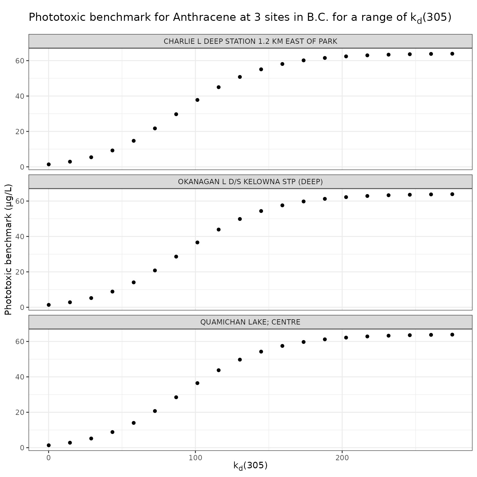
We will test the sensitivity to using sample values from Table 3 (Jourabchi (2023)), from 0.08 to 275:
Show/Hide Code
kd_vals <- seq(0.08, 275, length.out = 20)Effect of varying kd on phototoxic benchmark and ratio of phototoxic:narcotic benchmark for Anthracene
Show/Hide Code
kd_test_a <- multi_pb(
  sites,
  pah = "Anthracene",
  varying = "Kd_ref",
  vals = kd_vals,
  Kd_wvl = 305,
  o3_tc = 300,
  tauaer = 0.235
)

ggplot(kd_test_a, aes(x = Kd_ref, y = phototoxic_benchmark)) +
  geom_point() +
  facet_wrap(vars(name), ncol = 1) +
  labs(
    title = "Phototoxic benchmark for Anthracene at 3 sites in B.C. for a range of k~d~(305)",
    x = "k~d~(305)",
    y = "Phototoxic benchmark (μg/L)"
  )
Show/Hide Code
ggplot(kd_test_a, aes(x = Kd_ref, y = p_n_ratio)) +
  geom_point() +
  facet_wrap(vars(name), ncol = 1) +
  labs(
    title = "Ratio of phototoxic:narcotic benchmark for Anthracene at 3 sites in B.C. for a range of k~d~(305)",
    x = "k~d~(305)",
    y = "Ratio of phototoxic:narcotic benchmark"
  )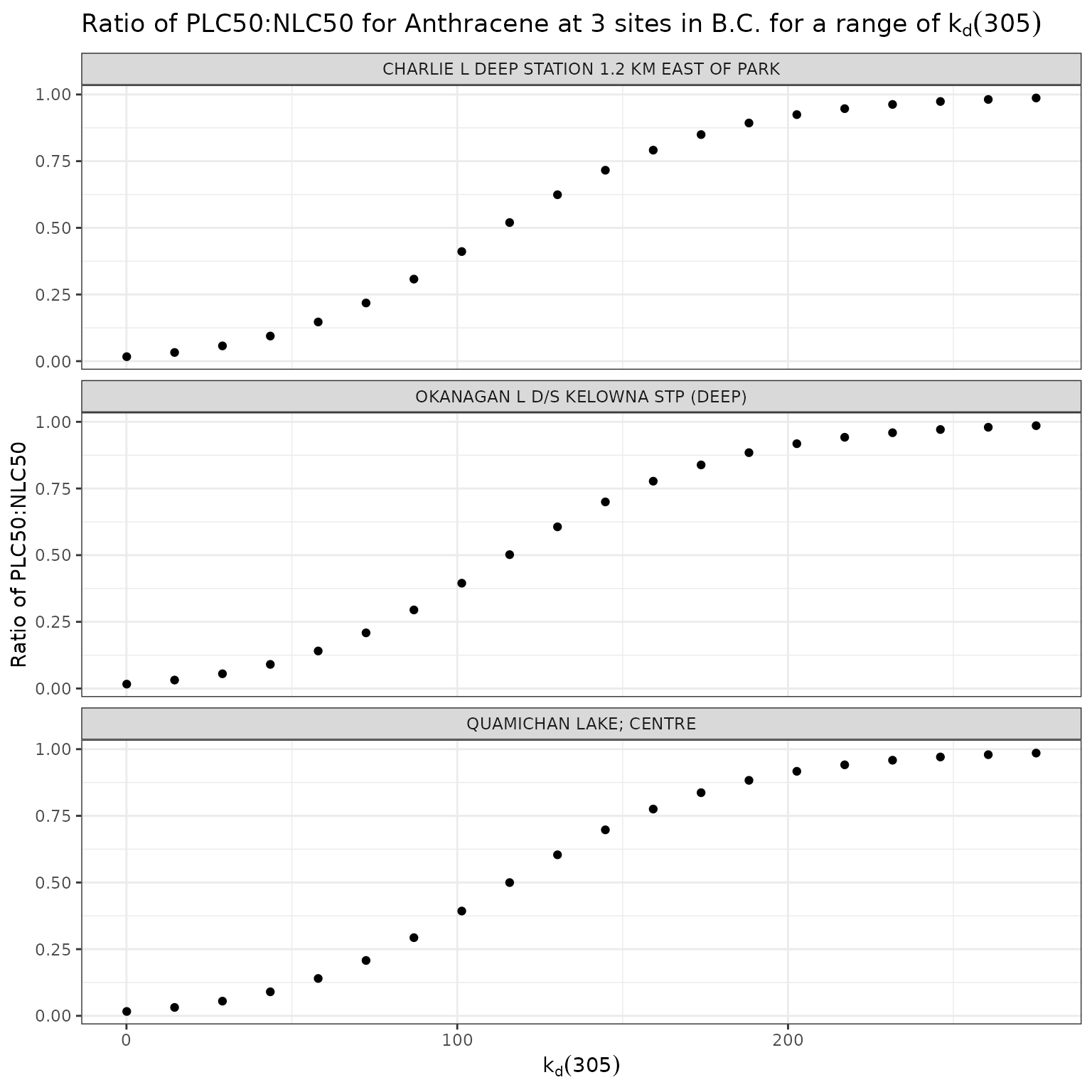
For Anthracene, the ratio of phototoxic:narcotic benchmark approaches 1 when is ~ 250 — in other words at that level of , phototoxic benchmark is nearly the same as narcotic benchmark, indicating that the light is attenuated to such an extent that the phototoxicity of Anthracene is not activated at the light levels when >= 250.
According to the above equation for estimating from [DOC]:
[DOC] ~= 56
Therefore of ~250 is representative of light attenuation when [DOC] is ~56. This is a significantly higher DOC concentration than observed in our three sample lakes, and is near the maximum of the range for which the above equation is recommended (it is recommended for [DOC] between 0.2 and 61.45 mg/L).
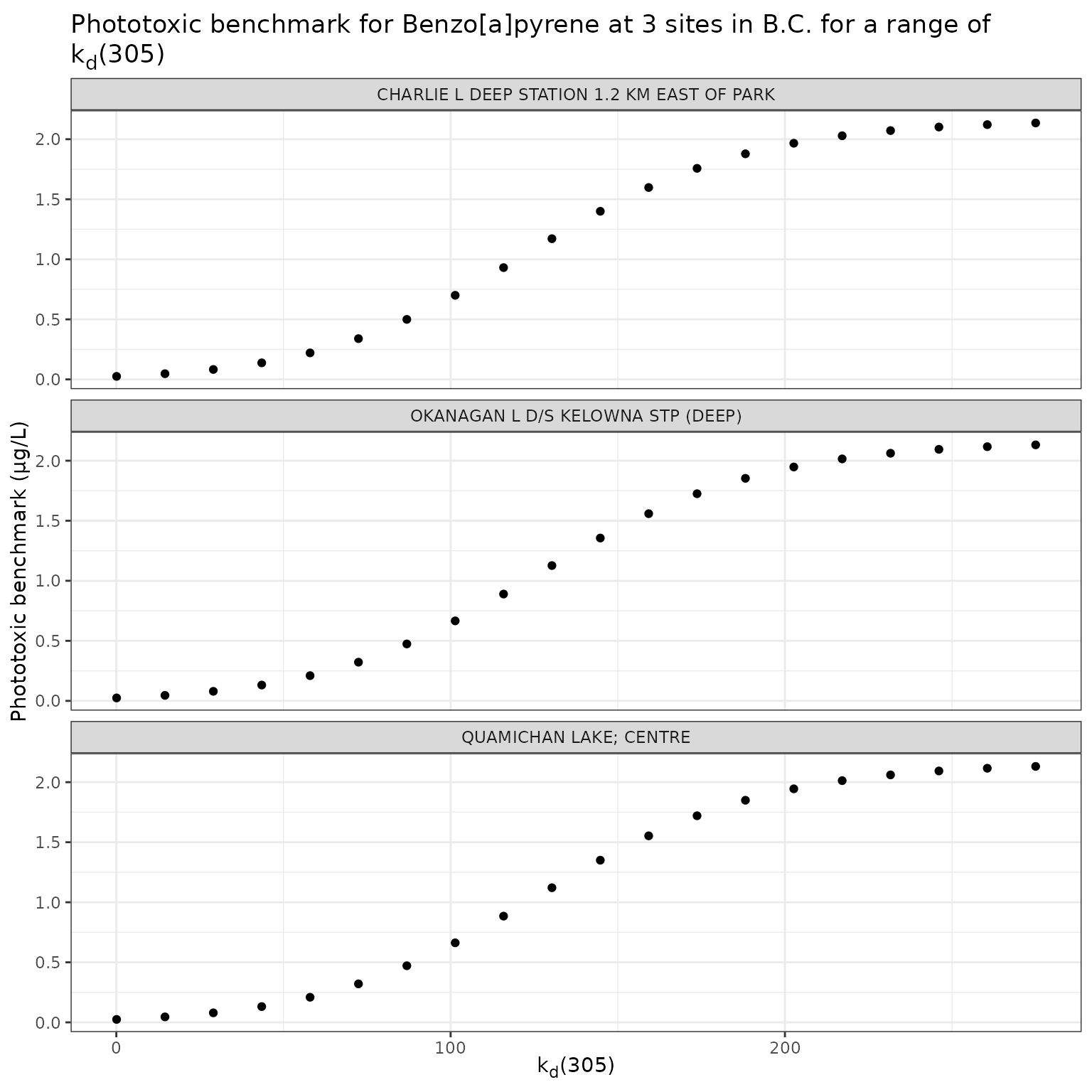
Effect of varying kd on phototoxic benchmark and ratio of phototoxic:narcotic benchmark for Benzo[a]pyrene
We will use the same input values as we did for Anthracene:
Show/Hide Code
kd_test_b <- multi_pb(
  sites,
  pah = "Benzo[a]pyrene",
  varying = "Kd_ref",
  vals = kd_vals,
  Kd_wvl = 305,
  o3_tc = 300,
  tauaer = 0.235
)

ggplot(kd_test_b, aes(x = Kd_ref, y = phototoxic_benchmark)) +
  geom_point() +
  facet_wrap(vars(name), ncol = 1) +
  labs(
    title = "Phototoxic benchmark for Benzo[a]pyrene at 3 sites in B.C. for a range of k~d~(305)",
    x = "k~d~(305)",
    y = "Phototoxic benchmark (μg/L)"
  )
Show/Hide Code
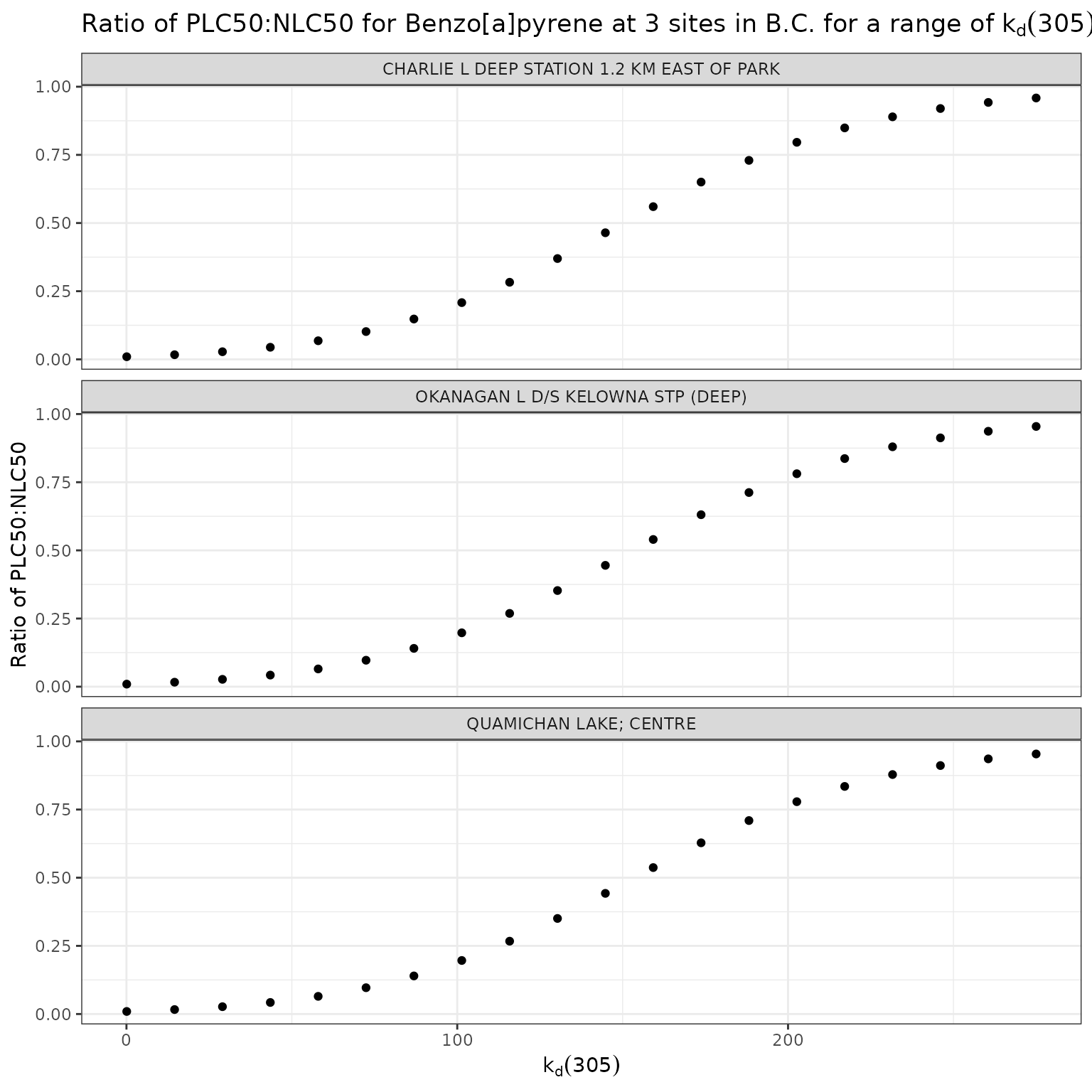
ggplot(kd_test_b, aes(x = Kd_ref, y = p_n_ratio)) +
  geom_point() +
  facet_wrap(vars(name), ncol = 1) +
  labs(
    title = "Ratio of phototoxic:narcotic benchmark for Benzo[a]pyrene at 3 sites in B.C. for a range of k~d~(305)",
    x = "k~d~(305)",
    y = "Ratio of phototoxic:narcotic benchmark"
  )
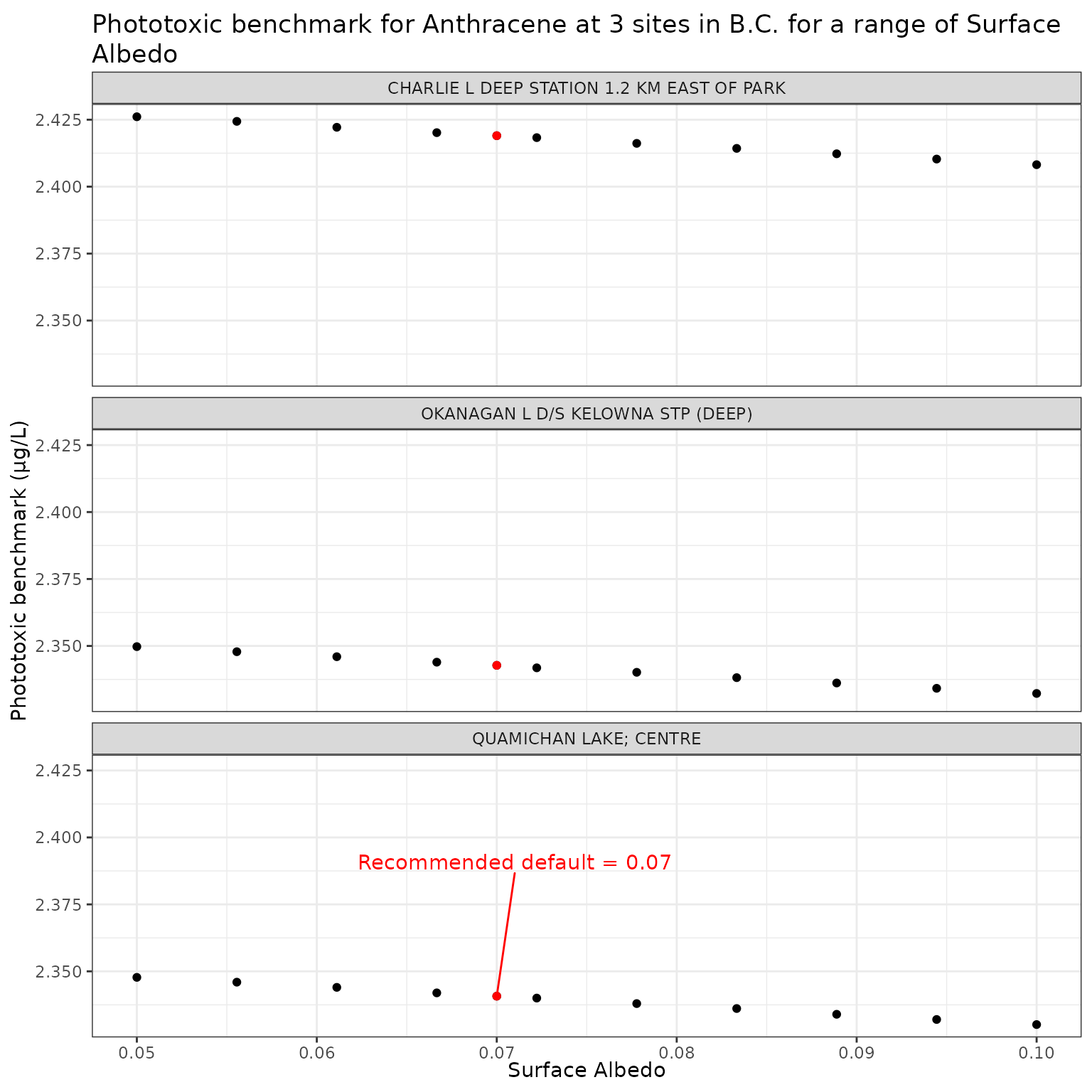
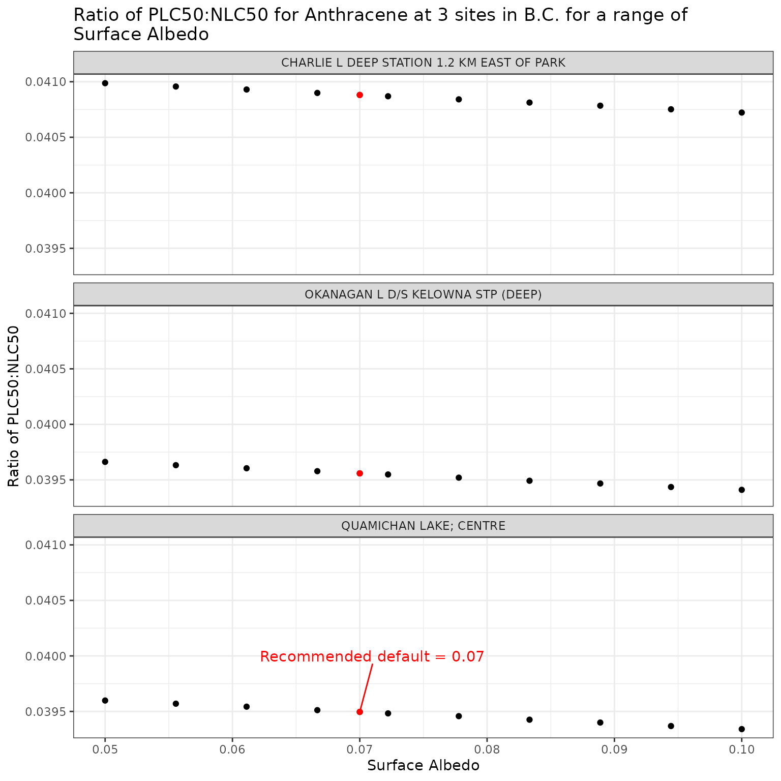
Surface Albedo (albedo)
We test surface albedo values from 0.05 to 0.1 (typical for water), and include the suggested default of 0.07:
For this and the remaining analyses, we will set DOC = 5 for all sites to ensure a constant value. We can then test the range of surface albedo values at all three sites for Anthracene and Benzo[a]pyrene.
Effect of varying Surface Albedo on phototoxic benchmark and ratio of phototoxic:narcotic benchmark for Anthracene
Show/Hide Code
albedo_test_a <- multi_pb(
  sites,
  pah = "Anthracene",
  varying = "albedo",
  vals = albedo_vals,
  DOC = 5,
  o3_tc = 300,
  tauaer = 0.235
)

ggplot(albedo_test_a, aes(x = albedo, y = phototoxic_benchmark)) +
  geom_point() +
  facet_wrap(vars(name), ncol = 1) +
  geom_point(
    data = filter(albedo_test_a, albedo == 0.07),
    colour = "red"
  ) +
  geom_text_repel(
    data = filter(
      albedo_test_a,
      albedo == 0.07,
      name == "QUAMICHAN LAKE; CENTRE"
    ),
    colour = "red",
    label = "Recommended default = 0.07",
    nudge_x = 0.001,
    nudge_y = 0.05
  ) +
  labs(
    title = "Phototoxic benchmark for Anthracene at 3 sites in B.C. for a range of Surface Albedo",
    x = "Surface Albedo",
    y = "Phototoxic benchmark (μg/L)"
  )
Show/Hide Code
ggplot(albedo_test_a, aes(x = albedo, y = p_n_ratio)) +
  geom_point() +
  facet_wrap(vars(name), ncol = 1) +
  geom_point(
    data = filter(albedo_test_a, albedo == 0.07),
    colour = "red"
  ) +
  geom_text_repel(
    data = filter(
      albedo_test_a,
      albedo == 0.07,
      name == "QUAMICHAN LAKE; CENTRE"
    ),
    colour = "red",
    label = "Recommended default = 0.07",
    nudge_x = 0.001,
    nudge_y = 0.0005
  ) +
  labs(
    title = "Ratio of phototoxic:narcotic benchmark for Anthracene at 3 sites in B.C. for a range of\nSurface Albedo",
    x = "Surface Albedo",
    y = "Ratio of phototoxic:narcotic benchmark"
  )
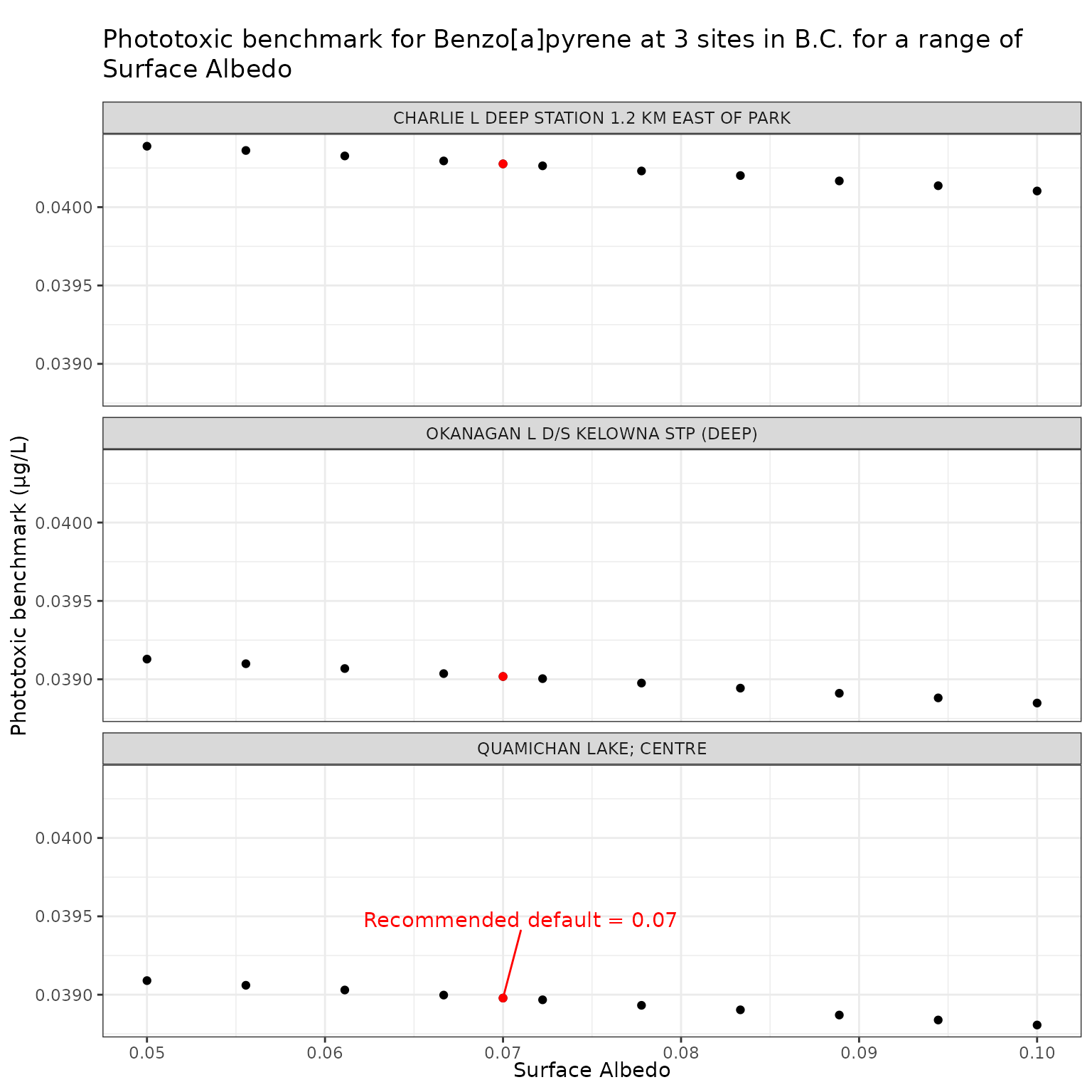
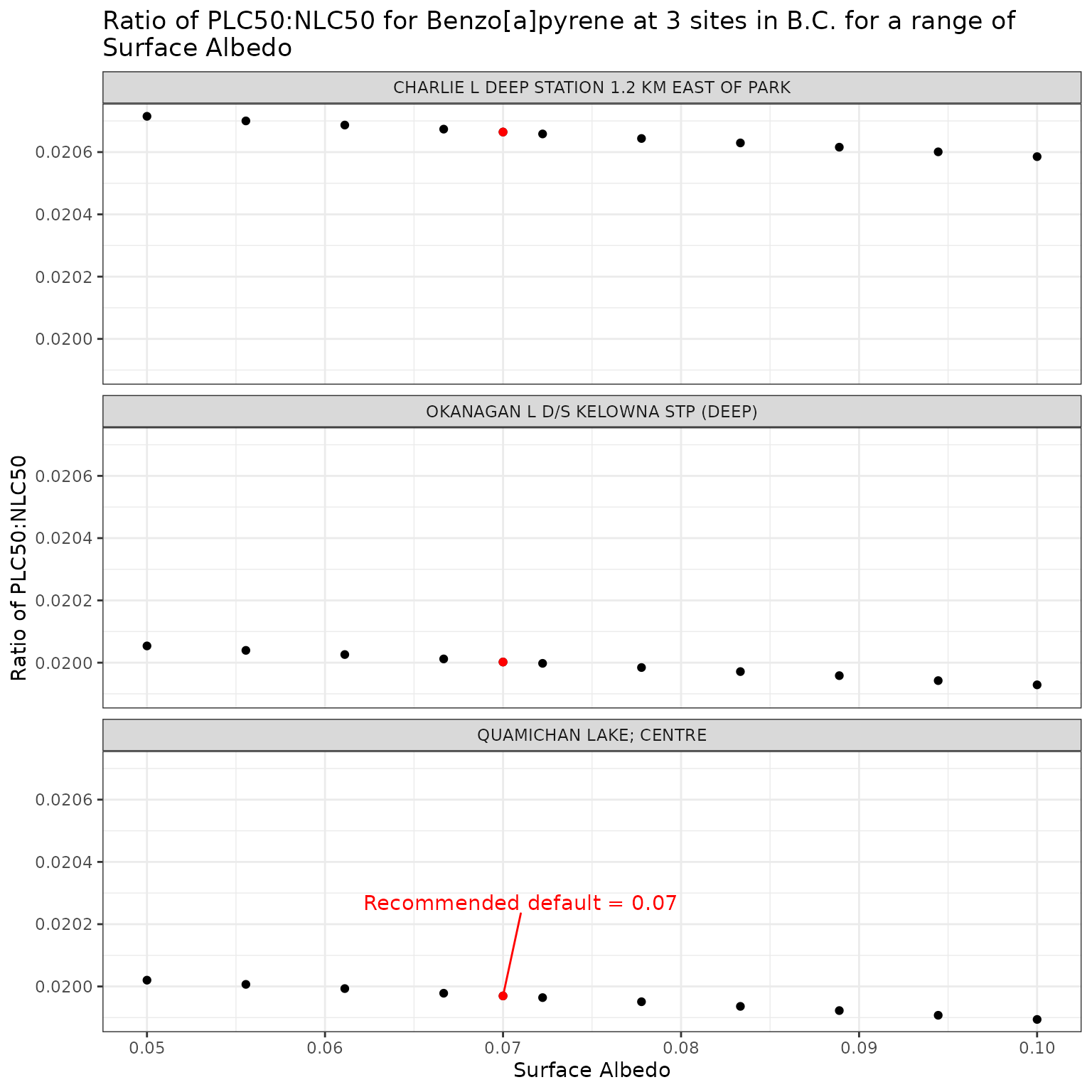
Effect of varying Surface Albedo on phototoxic benchmark and ratio of phototoxic:narcotic benchmark for Benzo[a]pyrene
Show/Hide Code
albedo_test_b <- multi_pb(
  sites,
  pah = "Benzo[a]pyrene",
  varying = "albedo",
  vals = albedo_vals,
  DOC = 5,
  o3_tc = 300,
  tauaer = 0.235
)

ggplot(albedo_test_b, aes(x = albedo, y = phototoxic_benchmark)) +
  geom_point() +
  facet_wrap(vars(name), ncol = 1) +
  geom_point(
    data = filter(albedo_test_b, albedo == 0.07),
    colour = "red"
  ) +
  geom_text_repel(
    data = filter(
      albedo_test_b,
      albedo == 0.07,
      name == "QUAMICHAN LAKE; CENTRE"
    ),
    colour = "red",
    label = "Recommended default = 0.07",
    nudge_x = 0.001,
    nudge_y = 0.0005
  ) +
  labs(
    title = "Phototoxic benchmark for Benzo[a]pyrene at 3 sites in B.C. for a range of Surface Albedo",
    x = "Surface Albedo",
    y = "Phototoxic benchmark (μg/L)"
  )
Show/Hide Code
ggplot(albedo_test_b, aes(x = albedo, y = p_n_ratio)) +
  geom_point() +
  facet_wrap(vars(name), ncol = 1) +
  geom_point(
    data = filter(albedo_test_b, albedo == 0.07),
    colour = "red"
  ) +
  geom_text_repel(
    data = filter(
      albedo_test_b,
      albedo == 0.07,
      name == "QUAMICHAN LAKE; CENTRE"
    ),
    colour = "red",
    label = "Recommended default = 0.07",
    nudge_x = 0.001,
    nudge_y = 0.0003
  ) +
  labs(
    title = "Ratio of phototoxic:narcotic benchmark for Benzo[a]pyrene at 3 sites in B.C. for a range of\nSurface Albedo",
    x = "Surface Albedo",
    y = "Ratio of phototoxic:narcotic benchmark"
  )
Ozone Column (o3_tc)
The pahwq package currently uses average monthly ozone column data
from 1980-1991 from Fortuin and Kelder
(1998), which is bundled with the TUV model. Based on latitude
and longitude and month, the ozone column value is looked up and
supplied to the TUV model. This default behaviour can be overridden by
supplying a value to the o3_tc argument in the
set_tuv_aq_params function. In the absence of
climatological data, the recommended default value is 300 DU (Jourabchi (2023)).
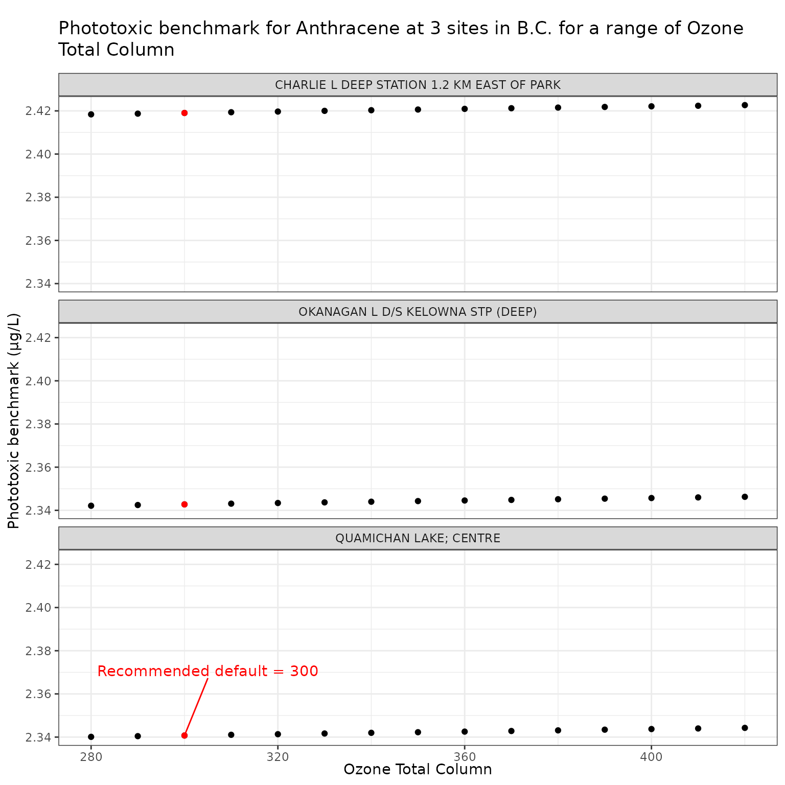
To test the sensitivity of phototoxic benchmark to ozone column, a range of values is tested from 280-420 DU, which are typical values in middle to Northern latitudes. See NASA’s ‘Ozone Watch’ page for more information on atmospheric ozone.
Show/Hide Code
ozone_vals <- seq(280, 420, by = 10)Effect of varying Ozone Total Column on phototoxic benchmark and ratio of phototoxic:narcotic benchmark for Anthracene
Show/Hide Code
ozone_test_a <- multi_pb(
  sites,
  pah = "Anthracene",
  varying = "o3_tc",
  vals = ozone_vals,
  DOC = 5,
  tauaer = 0.235
)

ggplot(ozone_test_a, aes(x = o3_tc, y = phototoxic_benchmark)) +
  geom_point() +
  facet_wrap(vars(name), ncol = 1) +
  geom_point(
    data = filter(ozone_test_a, o3_tc == 300),
    colour = "red"
  ) +
  geom_text_repel(
    data = filter(ozone_test_a, o3_tc == 300, name == "QUAMICHAN LAKE; CENTRE"),
    colour = "red",
    label = "Recommended default = 300",
    nudge_x = 5,
    nudge_y = 0.03
  ) +
  labs(
    title = "Phototoxic benchmark for Anthracene at 3 sites in B.C. for a range of Ozone Total Column",
    x = "Ozone Total Column",
    y = "Phototoxic benchmark (μg/L)"
  )
Show/Hide Code
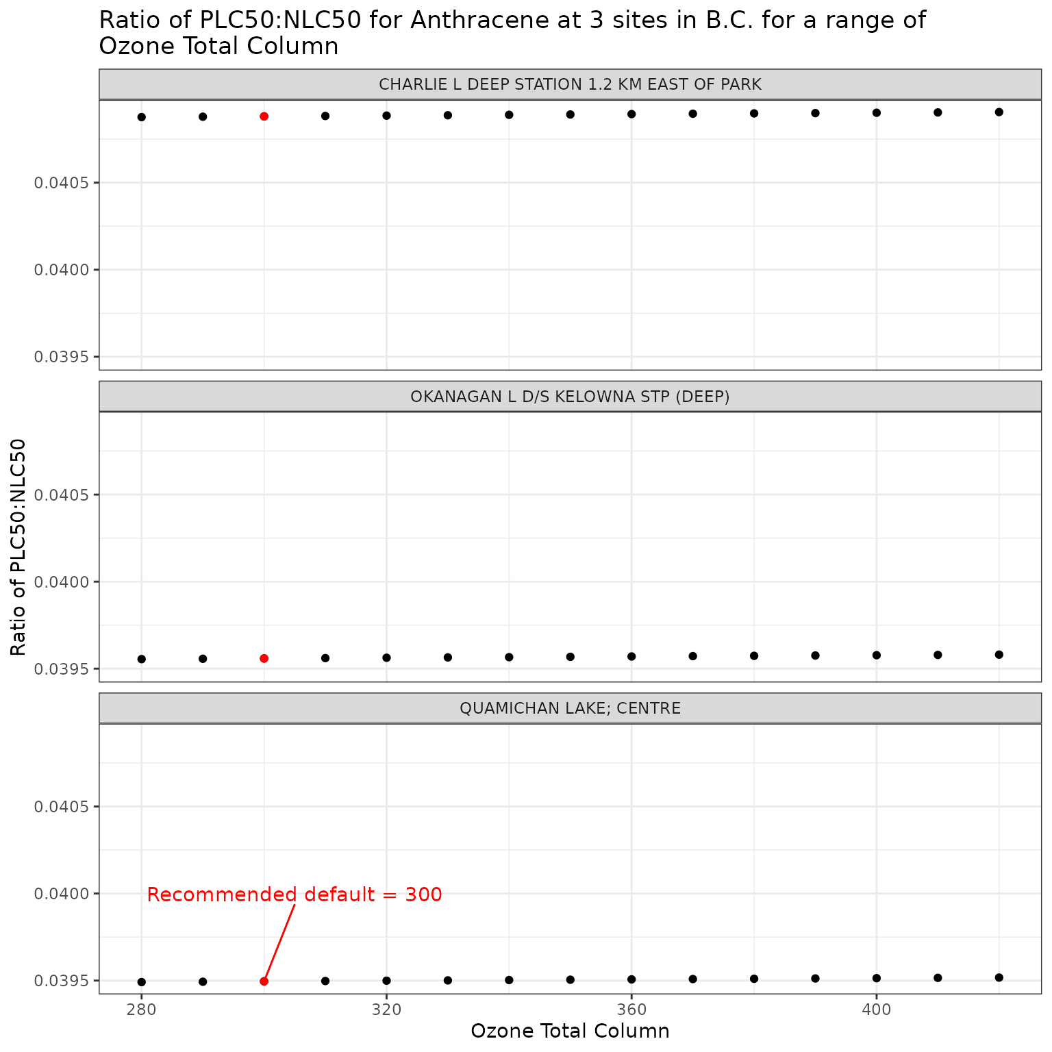
ggplot(ozone_test_a, aes(x = o3_tc, y = p_n_ratio)) +
  geom_point() +
  facet_wrap(vars(name), ncol = 1) +
  geom_point(
    data = filter(ozone_test_a, o3_tc == 300),
    colour = "red"
  ) +
  geom_text_repel(
    data = filter(ozone_test_a, o3_tc == 300, name == "QUAMICHAN LAKE; CENTRE"),
    colour = "red",
    label = "Recommended default = 300",
    nudge_x = 5,
    nudge_y = 0.0005
  ) +
  labs(
    title = "Ratio of phototoxic:narcotic benchmark for Anthracene at 3 sites in B.C. for a range of\nOzone Total Column",
    x = "Ozone Total Column",
    y = "Ratio of phototoxic:narcotic benchmark"
  )
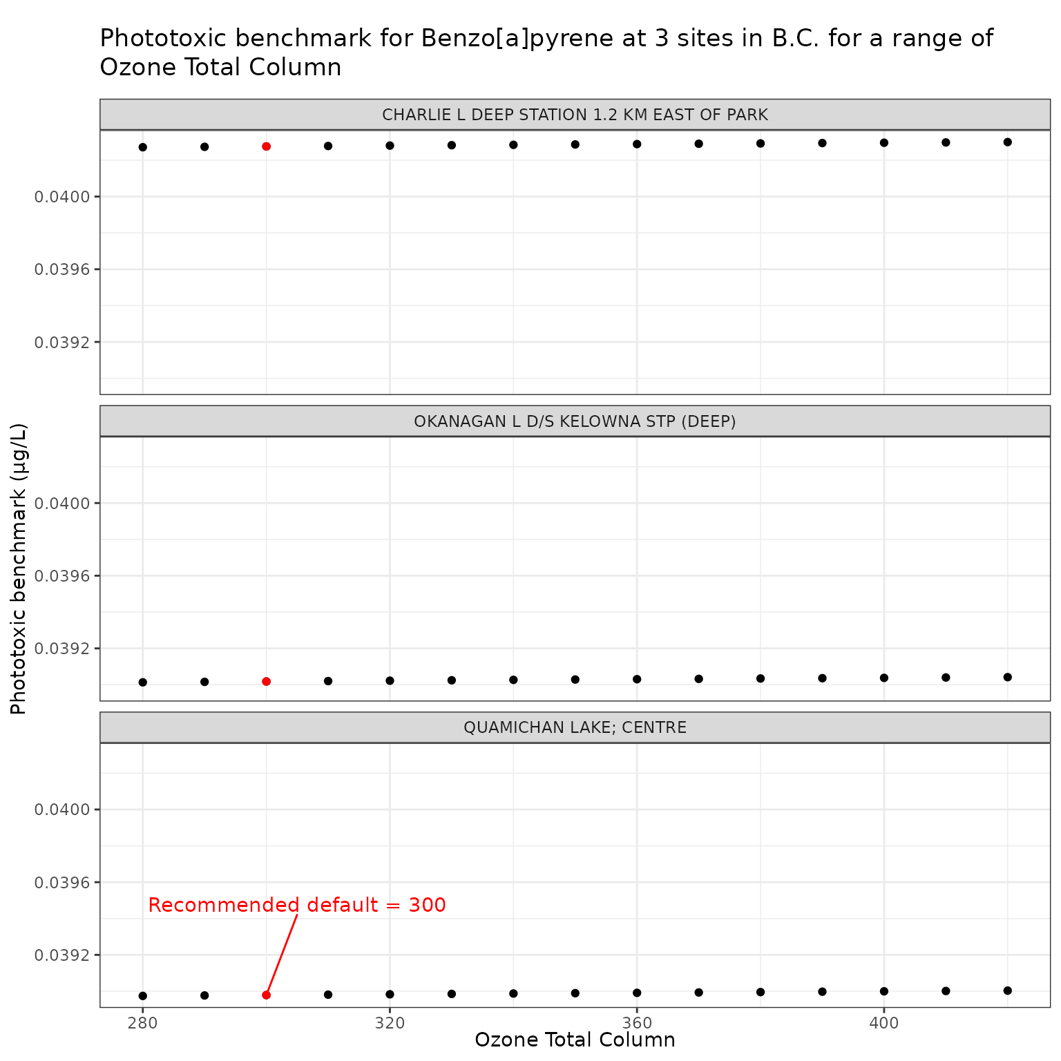
Effect of varying Ozone Total Column on phototoxic benchmark and ratio of phototoxic:narcotic benchmark for Benzo[a]pyrene
Show/Hide Code
ozone_test_b <- multi_pb(
  sites,
  pah = "Benzo[a]pyrene",
  varying = "o3_tc",
  vals = ozone_vals,
  DOC = 5,
  tauaer = 0.235
)

ggplot(ozone_test_b, aes(x = o3_tc, y = phototoxic_benchmark)) +
  geom_point() +
  facet_wrap(vars(name), ncol = 1) +
  geom_point(
    data = filter(ozone_test_b, o3_tc == 300),
    colour = "red"
  ) +
  geom_text_repel(
    data = filter(ozone_test_b, o3_tc == 300, name == "QUAMICHAN LAKE; CENTRE"),
    colour = "red",
    label = "Recommended default = 300",
    nudge_x = 5,
    nudge_y = 0.0005
  ) +
  labs(
    title = "Phototoxic benchmark for Benzo[a]pyrene at 3 sites in B.C. for a range of Ozone Total Column",
    x = "Ozone Total Column",
    y = "Phototoxic benchmark (μg/L)"
  )
Show/Hide Code
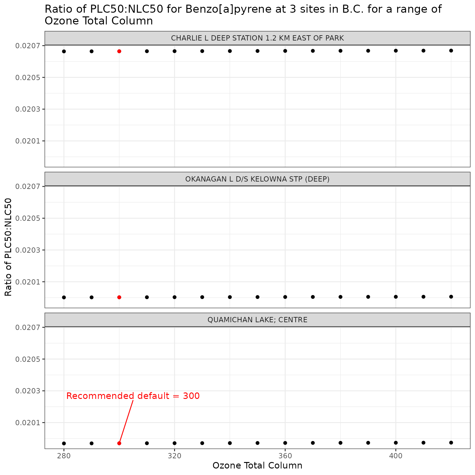
ggplot(ozone_test_b, aes(x = o3_tc, y = p_n_ratio)) +
  geom_point() +
  facet_wrap(vars(name), ncol = 1) +
  geom_point(
    data = filter(ozone_test_b, o3_tc == 300),
    colour = "red"
  ) +
  geom_text_repel(
    data = filter(ozone_test_b, o3_tc == 300, name == "QUAMICHAN LAKE; CENTRE"),
    colour = "red",
    label = "Recommended default = 300",
    nudge_x = 5,
    nudge_y = 0.0003
  ) +
  labs(
    title = "Ratio of phototoxic:narcotic benchmark for Benzo[a]pyrene at 3 sites in B.C. for a range of\nOzone Total Column",
    x = "Ozone Total Column",
    y = "Ratio of phototoxic:narcotic benchmark"
  )
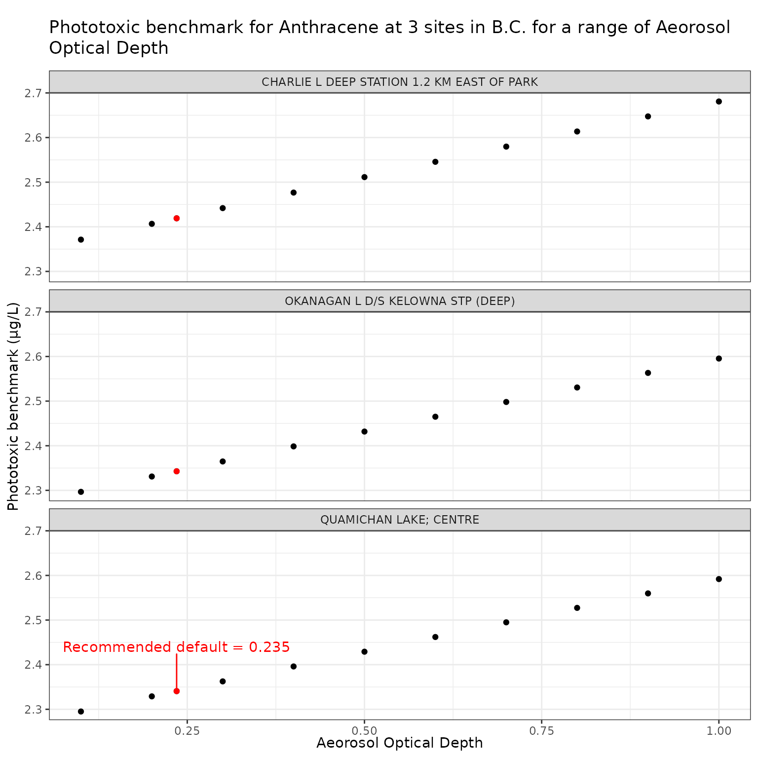
Aerosol Optical Depth (tauaer)
The pahwq package currently uses average monthly aerosol optical
depth data from 2002 to 2023, obtained from MODIS/Aqua satellite data.
Based on latitude and longitude and month, the AOD value is looked up
and supplied to the TUV model. This default behaviour can be overridden
by supplying a value to the tauaer argument in the
set_tuv_aq_params function. In the absence of
climatological data, the recommended default value is 0.235 (Jourabchi (2023)).
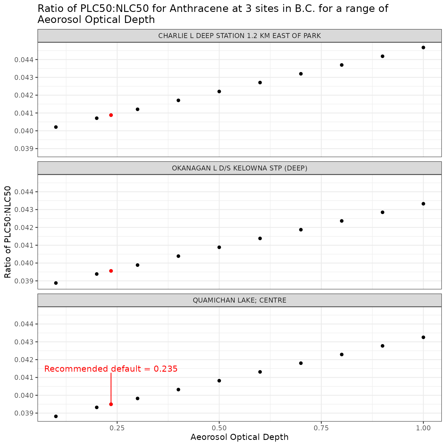
To test the sensitivity of phototoxic benchmark to AOD, a range of values is tested from 0.1 (clear skies with maximum visibility) to 1.0 (very hazy skies). See the NASA Earth Observatory page on aerosols.
Effect of Varying Aerosol Optical Depth (AOD) on phototoxic benchmark and ratio of phototoxic:narcotic benchmark for Anthracene
Show/Hide Code
aod_test_a <- multi_pb(
  sites,
  pah = "Anthracene",
  varying = "tauaer",
  vals = aod_vals,
  DOC = 5,
  o3_tc = 300
)

ggplot(aod_test_a, aes(x = tauaer, y = phototoxic_benchmark)) +
  geom_point() +
  facet_wrap(vars(name), ncol = 1) +
  geom_point(
    data = filter(aod_test_a, tauaer == 0.235),
    colour = "red"
  ) +
  geom_text_repel(
    data = filter(
      aod_test_a,
      tauaer == 0.235,
      name == "QUAMICHAN LAKE; CENTRE"
    ),
    colour = "red",
    label = "Recommended default = 0.235",
    nudge_y = 0.1
  ) +
  labs(
    title = "Phototoxic benchmark for Anthracene at 3 sites in B.C. for a range of Aeorosol Optical Depth",
    x = "Aeorosol Optical Depth",
    y = "Phototoxic benchmark (μg/L)"
  )
Show/Hide Code
ggplot(aod_test_a, aes(x = tauaer, y = p_n_ratio)) +
  geom_point() +
  facet_wrap(vars(name), ncol = 1) +
  geom_point(
    data = filter(aod_test_a, tauaer == 0.235),
    colour = "red"
  ) +
  geom_text_repel(
    data = filter(
      aod_test_a,
      tauaer == 0.235,
      name == "QUAMICHAN LAKE; CENTRE"
    ),
    colour = "red",
    label = "Recommended default = 0.235",
    nudge_y = 0.002
  ) +
  labs(
    title = "Ratio of phototoxic:narcotic benchmark for Anthracene at 3 sites in B.C. for a range of\nAeorosol Optical Depth",
    x = "Aeorosol Optical Depth",
    y = "Ratio of phototoxic:narcotic benchmark"
  )
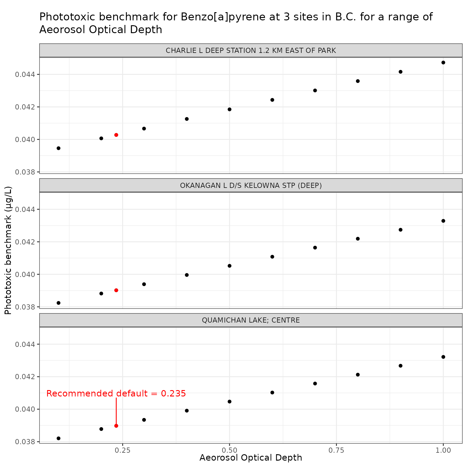
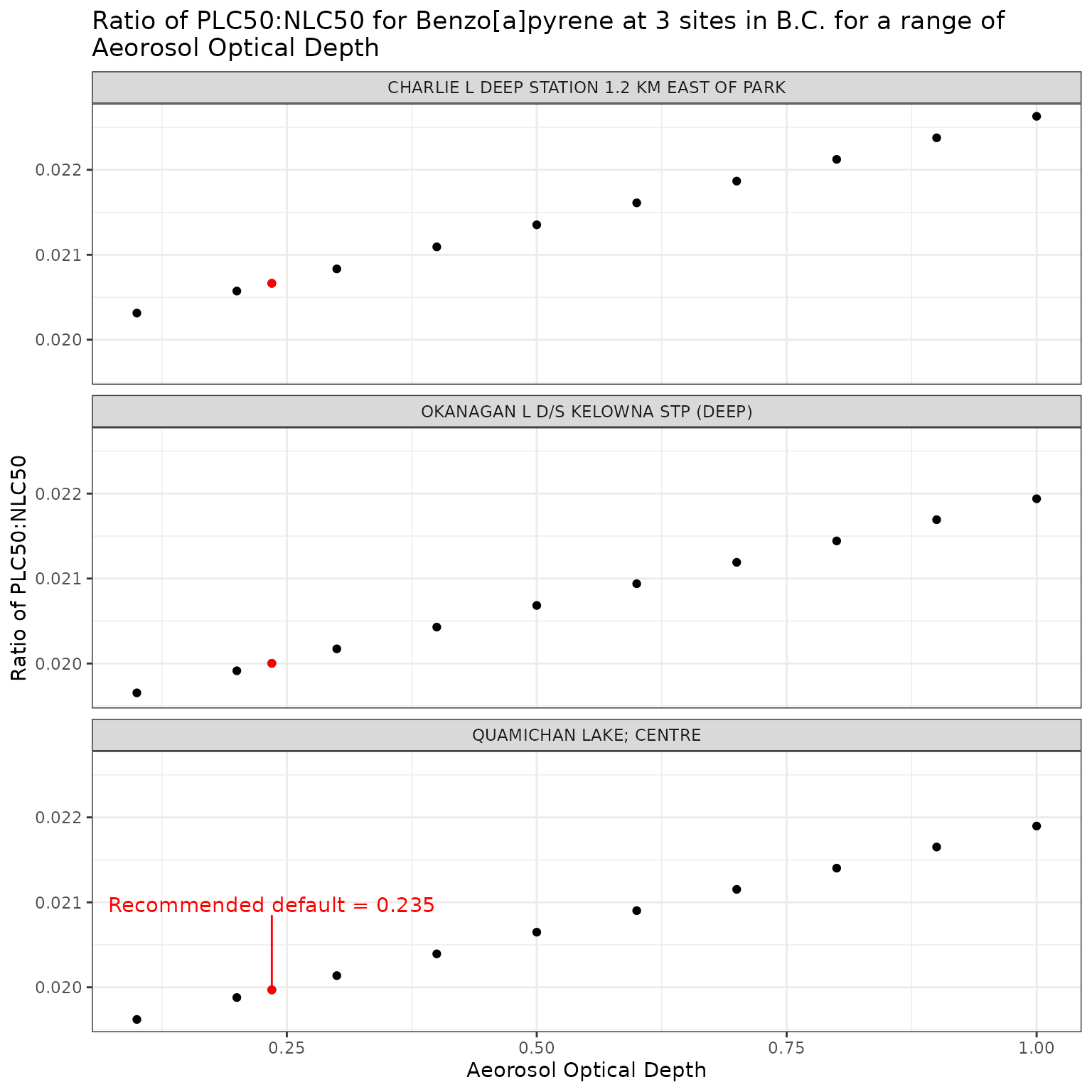
Effect of varying Aerosol Optical Depth (AOD) on phototoxic benchmark and ratio of phototoxic:narcotic benchmark for Benzo[a]pyrene
Show/Hide Code
aod_test_b <- multi_pb(
  sites,
  pah = "Benzo[a]pyrene",
  varying = "tauaer",
  vals = aod_vals,
  DOC = 5,
  o3_tc = 300
)

ggplot(aod_test_b, aes(x = tauaer, y = phototoxic_benchmark)) +
  geom_point() +
  facet_wrap(vars(name), ncol = 1) +
  geom_point(
    data = filter(aod_test_b, tauaer == 0.235),
    colour = "red"
  ) +
  geom_text_repel(
    data = filter(
      aod_test_b,
      tauaer == 0.235,
      name == "QUAMICHAN LAKE; CENTRE"
    ),
    colour = "red",
    label = "Recommended default = 0.235",
    nudge_y = 0.002
  ) +
  labs(
    title = "Phototoxic benchmark for Benzo[a]pyrene at 3 sites in B.C. for a range of\nAeorosol Optical Depth",
    x = "Aeorosol Optical Depth",
    y = "Phototoxic benchmark (μg/L)"
  )
Show/Hide Code
ggplot(aod_test_b, aes(x = tauaer, y = p_n_ratio)) +
  geom_point() +
  facet_wrap(vars(name), ncol = 1) +
  geom_point(
    data = filter(aod_test_b, tauaer == 0.235),
    colour = "red"
  ) +
  geom_text_repel(
    data = filter(
      aod_test_b,
      tauaer == 0.235,
      name == "QUAMICHAN LAKE; CENTRE"
    ),
    colour = "red",
    label = "Recommended default = 0.235",
    nudge_y = 0.001
  ) +
  labs(
    title = "Ratio of phototoxic:narcotic benchmark for Benzo[a]pyrene at 3 sites in B.C. for a range of\nAeorosol Optical Depth",
    x = "Aeorosol Optical Depth",
    y = "Ratio of phototoxic:narcotic benchmark"
  )
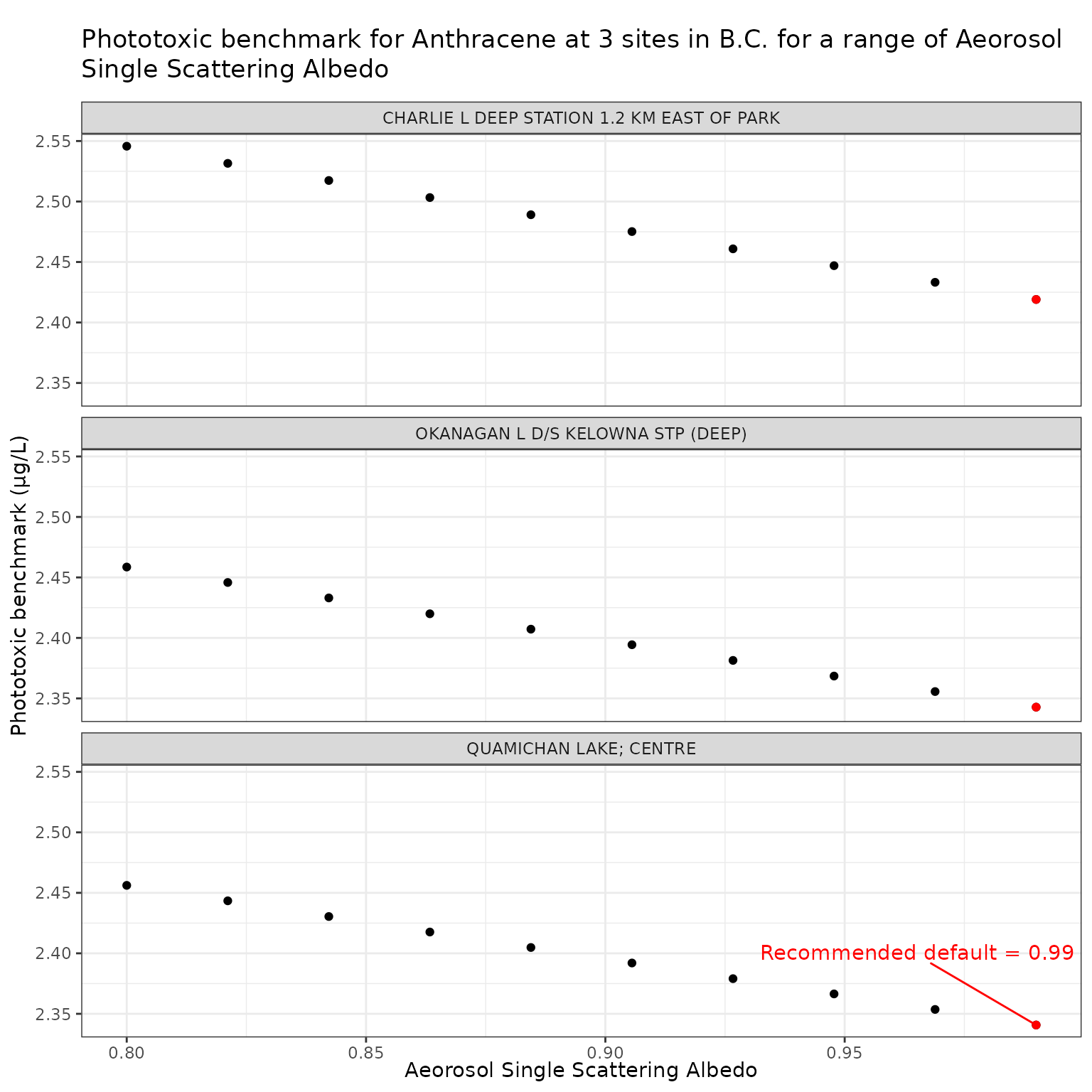
Aerosol Single Scattering Albedo (ssaaer)
Aerosol Single Scattering Albedo is currently set as a default
constant value of 0.99. This can be overridden by setting the
ssaaer parameter of the set_tuv_aq_params()
function to a different value.
Here we test a range for values from 0.80 to 0.99, including the recommended default of 0.99 (Jourabchi (2023)).
Show/Hide Code
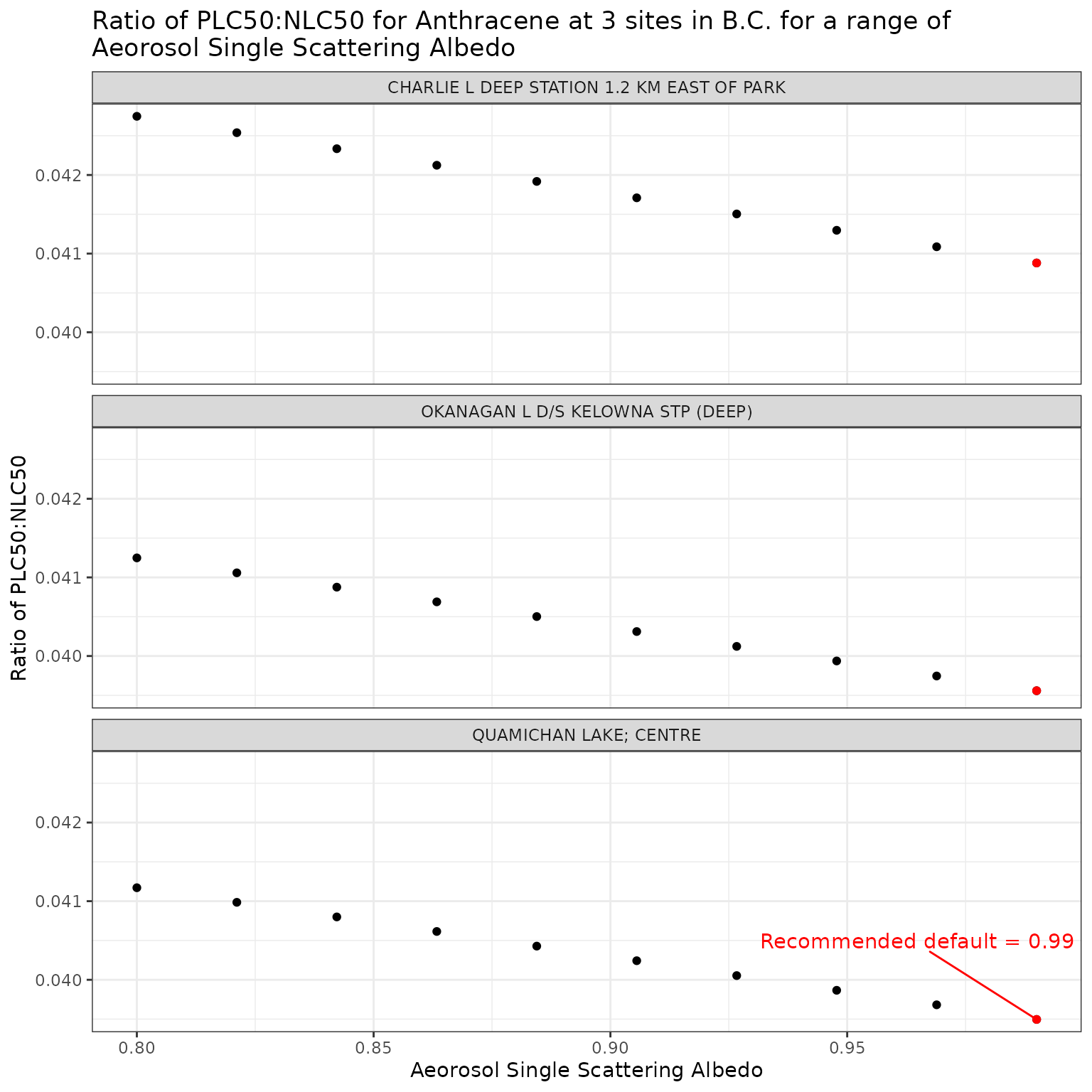
ssa_vals <- seq(0.8, 0.99, length.out = 10)Effect of varying Aerosol Single Scattering Albedo on phototoxic benchmark and ratio of phototoxic:narcotic benchmark for Anthracene
Show/Hide Code
ssa_test_a <- multi_pb(
  sites,
  pah = "Anthracene",
  varying = "ssaaer",
  vals = ssa_vals,
  DOC = 5,
  o3_tc = 300,
  tauaer = 0.235
)

ggplot(ssa_test_a, aes(x = ssaaer, y = phototoxic_benchmark)) +
  geom_point() +
  facet_wrap(vars(name), ncol = 1) +
  geom_point(
    data = filter(ssa_test_a, ssaaer == 0.99),
    colour = "red"
  ) +
  geom_text_repel(
    data = filter(ssa_test_a, ssaaer == 0.99, name == "QUAMICHAN LAKE; CENTRE"),
    colour = "red",
    label = "Recommended default = 0.99",
    nudge_y = .06
  ) +
  labs(
    title = "Phototoxic benchmark for Anthracene at 3 sites in B.C. for a range of\nAeorosol Single Scattering Albedo",
    x = "Aeorosol Single Scattering Albedo",
    y = "Phototoxic benchmark (μg/L)"
  )
Show/Hide Code
ggplot(ssa_test_a, aes(x = ssaaer, y = p_n_ratio)) +
  geom_point() +
  facet_wrap(vars(name), ncol = 1) +
  geom_point(
    data = filter(ssa_test_a, ssaaer == 0.99),
    colour = "red"
  ) +
  geom_text_repel(
    data = filter(ssa_test_a, ssaaer == 0.99, name == "QUAMICHAN LAKE; CENTRE"),
    colour = "red",
    label = "Recommended default = 0.99",
    nudge_y = .001
  ) +
  labs(
    title = "Ratio of phototoxic:narcotic benchmark for Anthracene at 3 sites in B.C. for a range of\nAeorosol Single Scattering Albedo",
    x = "Aeorosol Single Scattering Albedo",
    y = "Ratio of phototoxic:narcotic benchmark"
  )
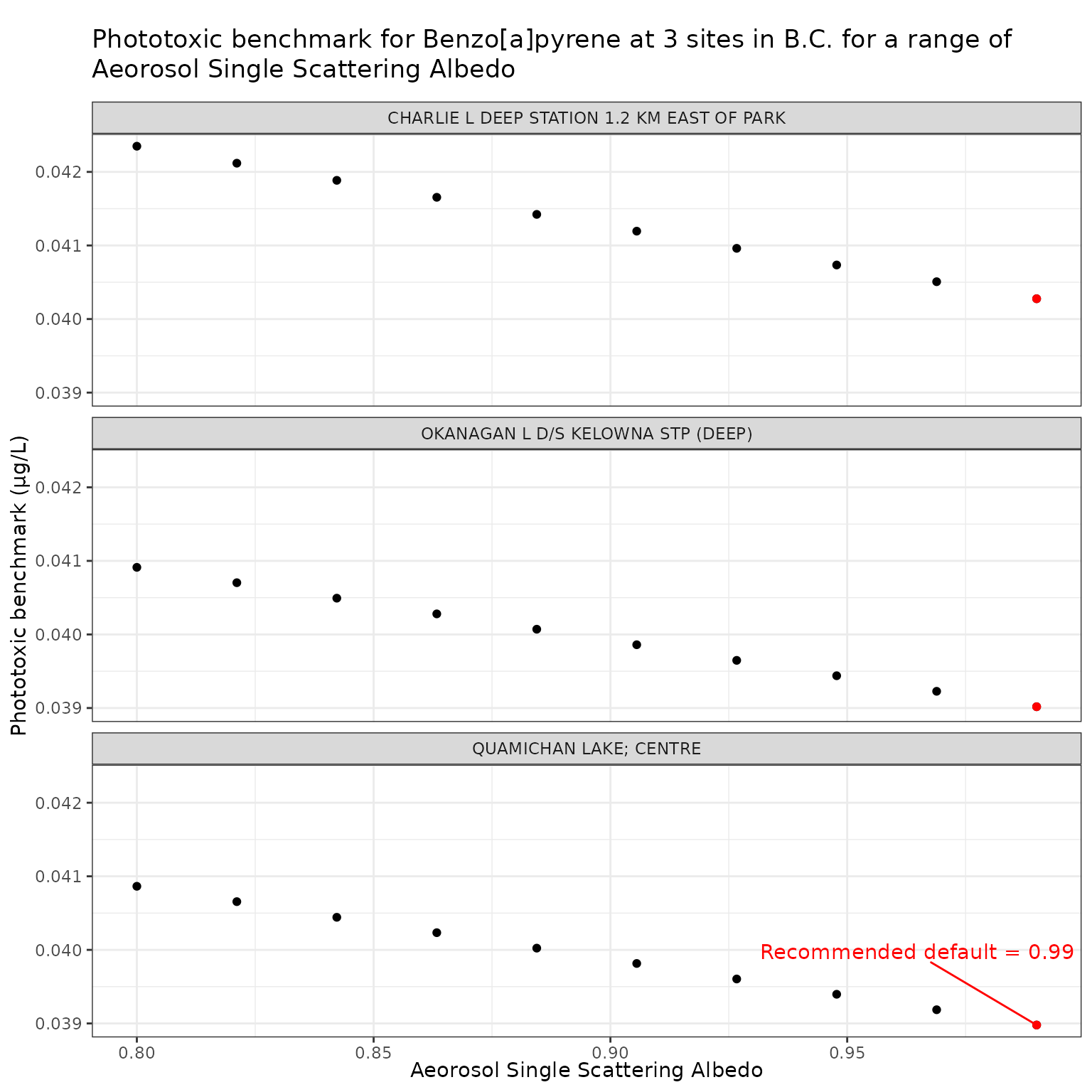
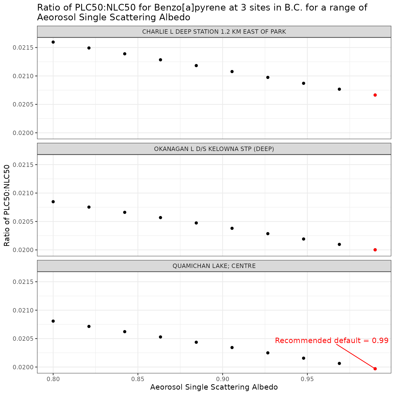
Effect of varying Aerosol Single Scattering Albedo on phototoxic benchmark and ratio of phototoxic:narcotic benchmark for Benzo[a]pyrene
Show/Hide Code
ssa_test_b <- multi_pb(
  sites,
  pah = "Benzo[a]pyrene",
  varying = "ssaaer",
  vals = ssa_vals,
  DOC = 5,
  o3_tc = 300,
  tauaer = 0.235
)

ggplot(ssa_test_b, aes(x = ssaaer, y = phototoxic_benchmark)) +
  geom_point() +
  facet_wrap(vars(name), ncol = 1) +
  geom_point(
    data = filter(ssa_test_b, ssaaer == 0.99),
    colour = "red"
  ) +
  geom_text_repel(
    data = filter(ssa_test_b, ssaaer == 0.99, name == "QUAMICHAN LAKE; CENTRE"),
    colour = "red",
    label = "Recommended default = 0.99",
    nudge_y = .001
  ) +
  labs(
    title = "Phototoxic benchmark for Benzo[a]pyrene at 3 sites in B.C. for a range of\nAeorosol Single Scattering Albedo",
    x = "Aeorosol Single Scattering Albedo",
    y = "Phototoxic benchmark (μg/L)"
  )
Show/Hide Code
ggplot(ssa_test_b, aes(x = ssaaer, y = p_n_ratio)) +
  geom_point() +
  facet_wrap(vars(name), ncol = 1) +
  geom_point(
    data = filter(ssa_test_b, ssaaer == 0.99),
    colour = "red"
  ) +
  geom_text_repel(
    data = filter(ssa_test_b, ssaaer == 0.99, name == "QUAMICHAN LAKE; CENTRE"),
    colour = "red",
    label = "Recommended default = 0.99",
    nudge_y = .0005
  ) +
  labs(
    title = "Ratio of phototoxic:narcotic benchmark for Benzo[a]pyrene at 3 sites in B.C. for a range of\nAeorosol Single Scattering Albedo",
    x = "Aeorosol Single Scattering Albedo",
    y = "Ratio of phototoxic:narcotic benchmark"
  )
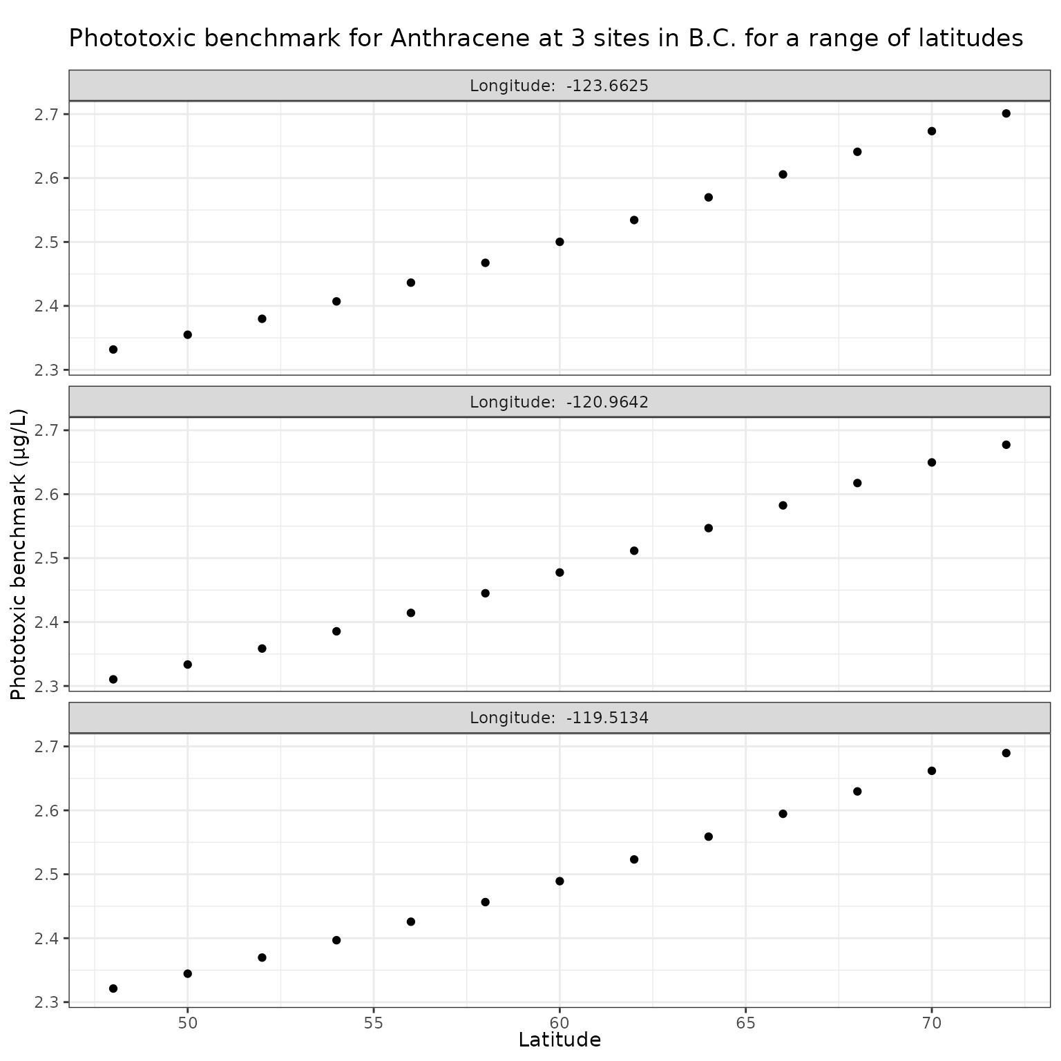
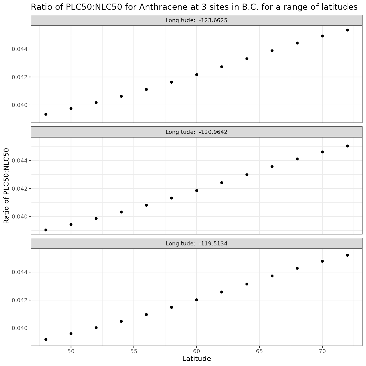
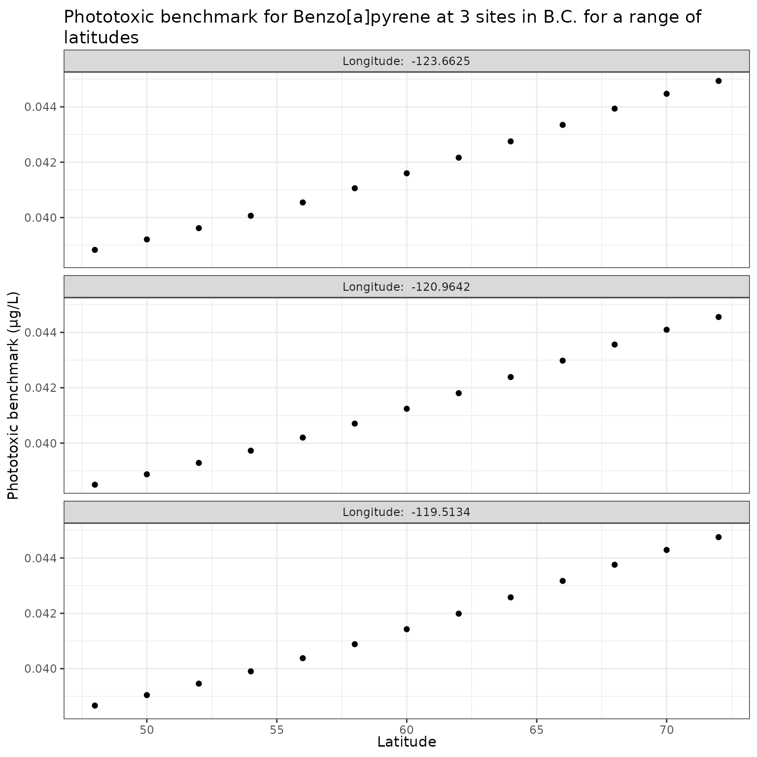
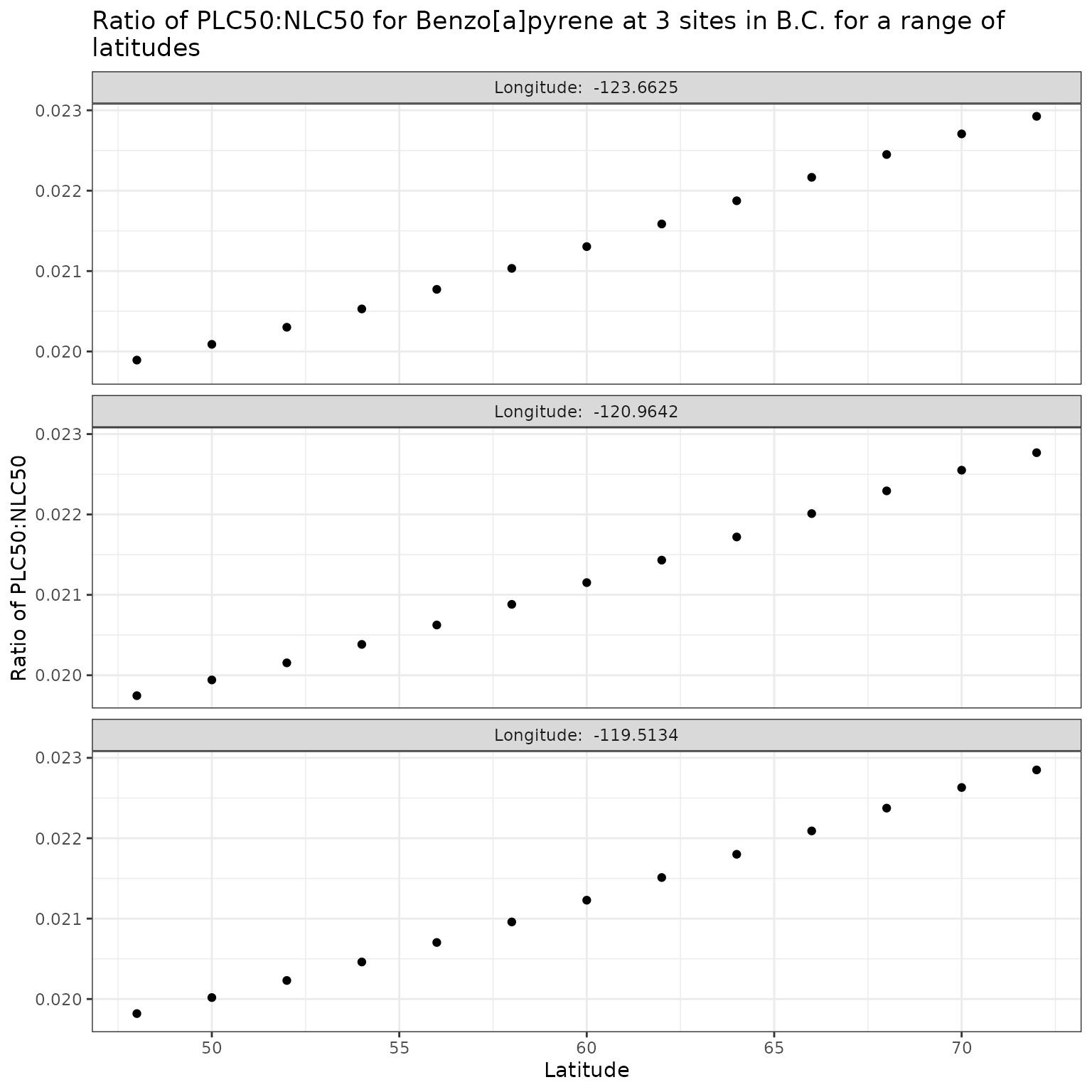
Latitude (lat)
Latitude has a strong effect on the angle of the sun, which will in turn affect the light penetration through water, thus it is important to investigate the sensitivity of the calculation of phototoxic benchmark to variation in latitude.
For this analysis, we will maintain the longitudes associated with each site, and make “mock” sites by creating a range of latitudes from 48 to 72 degrees N and pair those with the longitudes of the original sites.
lat_vals <- seq(48, 72, by = 2)Effect of varying Latitude on phototoxic benchmark and ratio of phototoxic:narcotic benchmark for Anthracene
Show/Hide Code
lat_test_a <- multi_pb(
  sites,
  pah = "Anthracene",
  varying = "lat",
  vals = lat_vals,
  DOC = 5,
  o3_tc = 300,
  tauaer = 0.235
)

ggplot(lat_test_a, aes(x = lat, y = phototoxic_benchmark)) +
  geom_point() +
  facet_wrap(
    vars(lon),
    ncol = 1,
    labeller = as_labeller(\(x) paste("Longitude: ", x))
  ) +
  labs(
    title = "Phototoxic benchmark for Anthracene at 3 sites in B.C. for a range of latitudes",
    x = "Latitude",
    y = "Phototoxic benchmark (μg/L)"
  )
Show/Hide Code
ggplot(lat_test_a, aes(x = lat, y = p_n_ratio)) +
  geom_point() +
  facet_wrap(
    vars(lon),
    ncol = 1,
    labeller = as_labeller(\(x) paste("Longitude: ", x))
  ) +
  labs(
    title = "Ratio of phototoxic:narcotic benchmark for Anthracene at 3 sites in B.C. for a range of latitudes",
    x = "Latitude",
    y = "Ratio of phototoxic:narcotic benchmark"
  )
Effect of varying Latitude on phototoxic benchmark and ratio of phototoxic:narcotic benchmark for Benzo[a]pyrene
Show/Hide Code
lat_test_b <- multi_pb(
  sites,
  pah = "Benzo[a]pyrene",
  varying = "lat",
  vals = lat_vals,
  DOC = 5,
  o3_tc = 300,
  tauaer = 0.235
)

ggplot(lat_test_b, aes(x = lat, y = phototoxic_benchmark)) +
  geom_point() +
  facet_wrap(
    vars(lon),
    ncol = 1,
    labeller = as_labeller(\(x) paste("Longitude: ", x))
  ) +
  labs(
    title = "Phototoxic benchmark for Benzo[a]pyrene at 3 sites in B.C. for a range of latitudes",
    x = "Latitude",
    y = "Phototoxic benchmark (μg/L)"
  )
Show/Hide Code
ggplot(lat_test_b, aes(x = lat, y = p_n_ratio)) +
  geom_point() +
  facet_wrap(
    vars(lon),
    ncol = 1,
    labeller = as_labeller(\(x) paste("Longitude: ", x))
  ) +
  labs(
    title = "Ratio of phototoxic:narcotic benchmark for Benzo[a]pyrene at 3 sites in B.C. for a range of\nlatitudes",
    x = "Latitude",
    y = "Ratio of phototoxic:narcotic benchmark"
  )
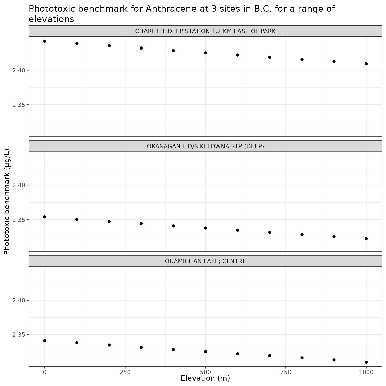
Elevation (elev_m)
We can test the effect of elevation on phototoxic benchmark by varying elevation from sea level to 1000m above sea level. We will keep the latitude and longitude associated with each site.
elevation_vals <- seq(0, 1000, by = 100)Effect of varying Elevation on phototoxic benchmark and ratio of phototoxic:narcotic benchmark for Anthracene
Show/Hide Code
elev_test_a <- multi_pb(
  sites,
  pah = "Anthracene",
  varying = "elev_m",
  vals = elevation_vals,
  DOC = 5,
  o3_tc = 300,
  tauaer = 0.235
)

ggplot(elev_test_a, aes(x = elev_m, y = phototoxic_benchmark)) +
  geom_point() +
  facet_wrap(vars(name), ncol = 1) +
  labs(
    title = "Phototoxic benchmark for Anthracene at 3 sites in B.C. for a range of elevations",
    x = "Elevation (m)",
    y = "Phototoxic benchmark (μg/L)"
  )
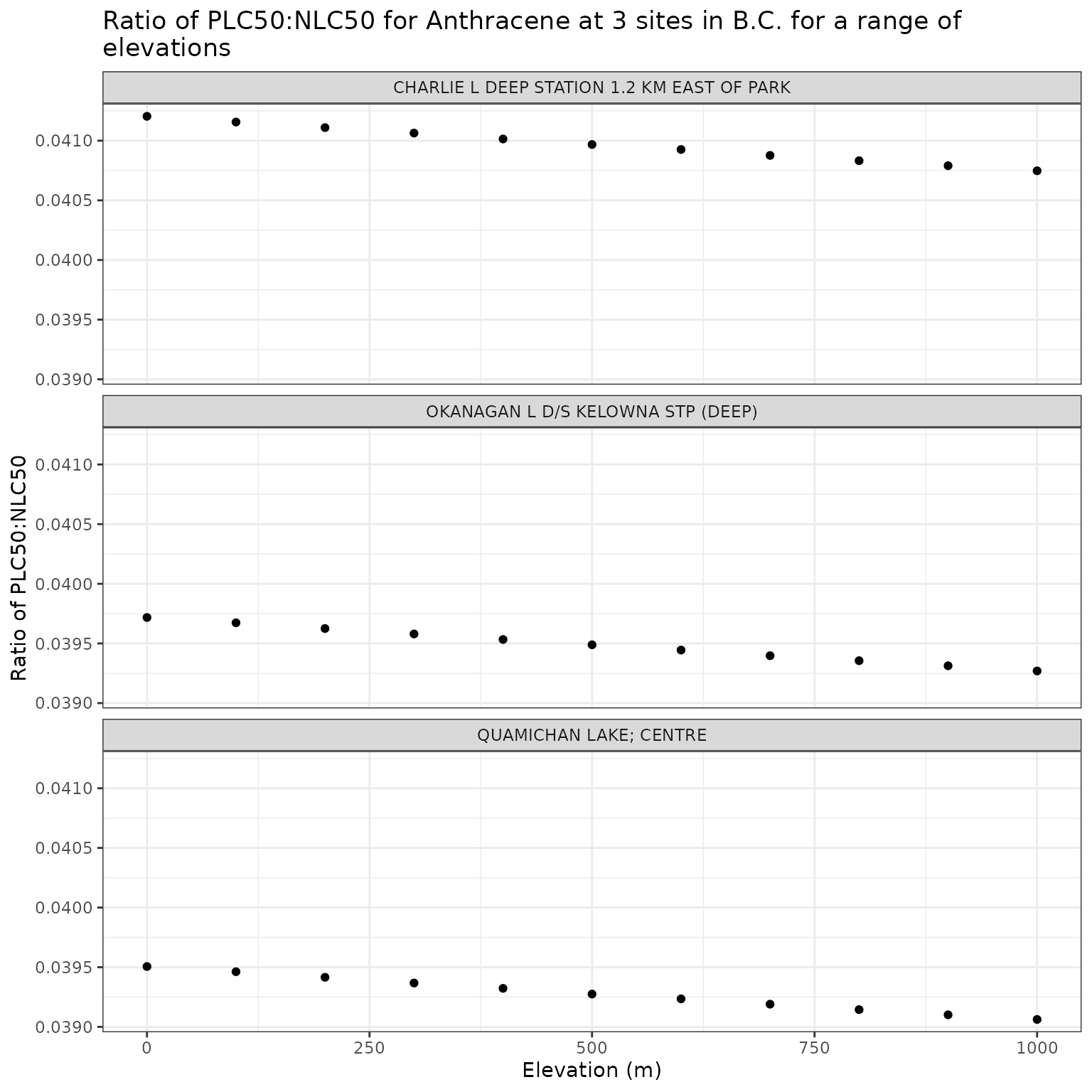
Show/Hide Code
ggplot(elev_test_a, aes(x = elev_m, y = p_n_ratio)) +
  geom_point() +
  facet_wrap(vars(name), ncol = 1) +
  labs(
    title = "Ratio of phototoxic:narcotic benchmark for Anthracene at 3 sites in B.C. for a range of\nelevations",
    x = "Elevation (m)",
    y = "Ratio of phototoxic:narcotic benchmark"
  )
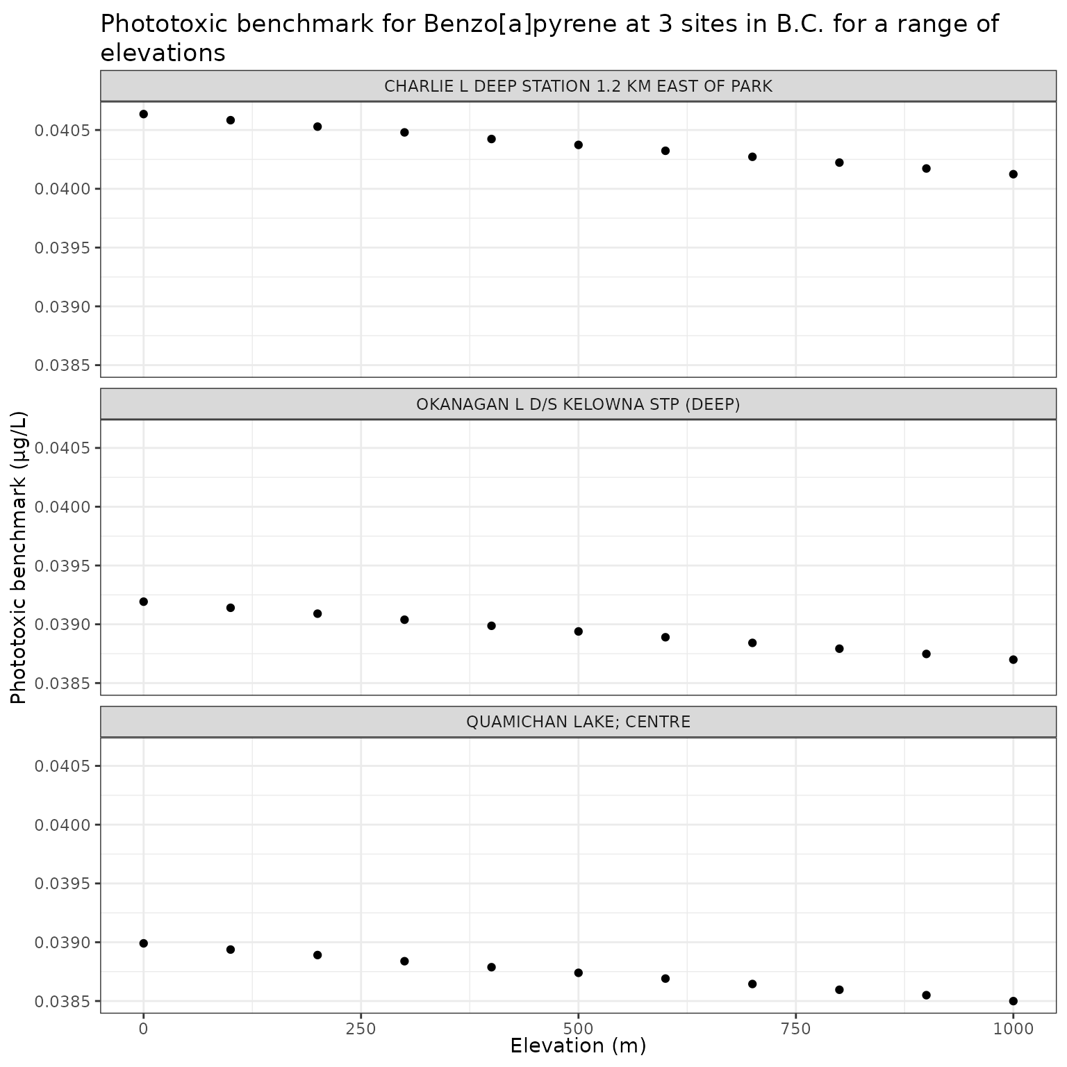
Effect of varying Elevation on phototoxic benchmark and ratio of phototoxic:narcotic benchmark for Benzo[a]pyrene
Show/Hide Code
elev_test_b <- multi_pb(
  sites,
  pah = "Benzo[a]pyrene",
  varying = "elev_m",
  vals = elevation_vals,
  DOC = 5,
  o3_tc = 300,
  tauaer = 0.235
)

ggplot(elev_test_b, aes(x = elev_m, y = phototoxic_benchmark)) +
  geom_point() +
  facet_wrap(vars(name), ncol = 1) +
  labs(
    title = "Phototoxic benchmark for Benzo[a]pyrene at 3 sites in B.C. for a range of elevations",
    x = "Elevation (m)",
    y = "Phototoxic benchmark (μg/L)"
  )
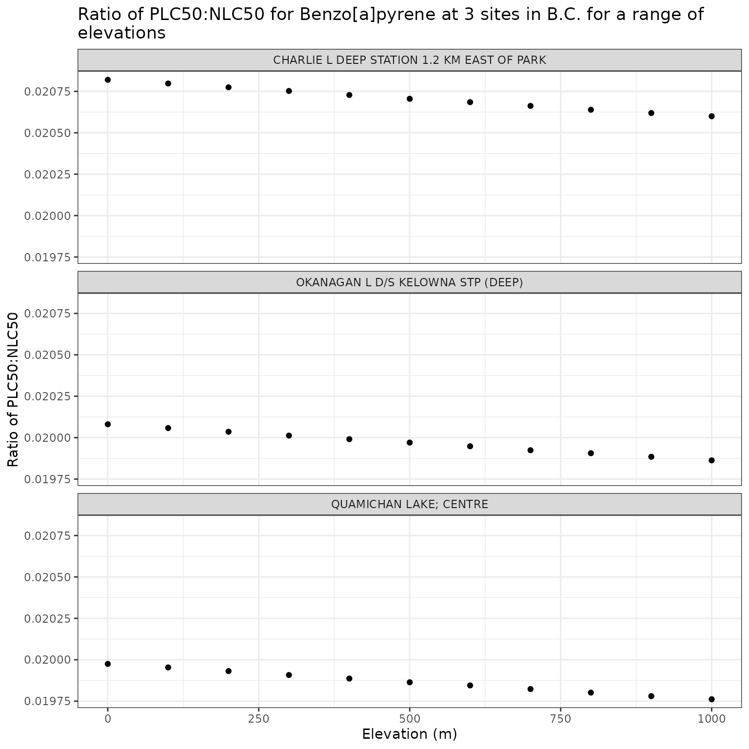
Show/Hide Code
ggplot(elev_test_b, aes(x = elev_m, y = p_n_ratio)) +
  geom_point() +
  facet_wrap(vars(name), ncol = 1) +
  labs(
    title = "Ratio of phototoxic:narcotic benchmark for Benzo[a]pyrene at 3 sites in B.C. for a range of\nelevations",
    x = "Elevation (m)",
    y = "Ratio of phototoxic:narcotic benchmark"
  )
Water depth (depth_m)
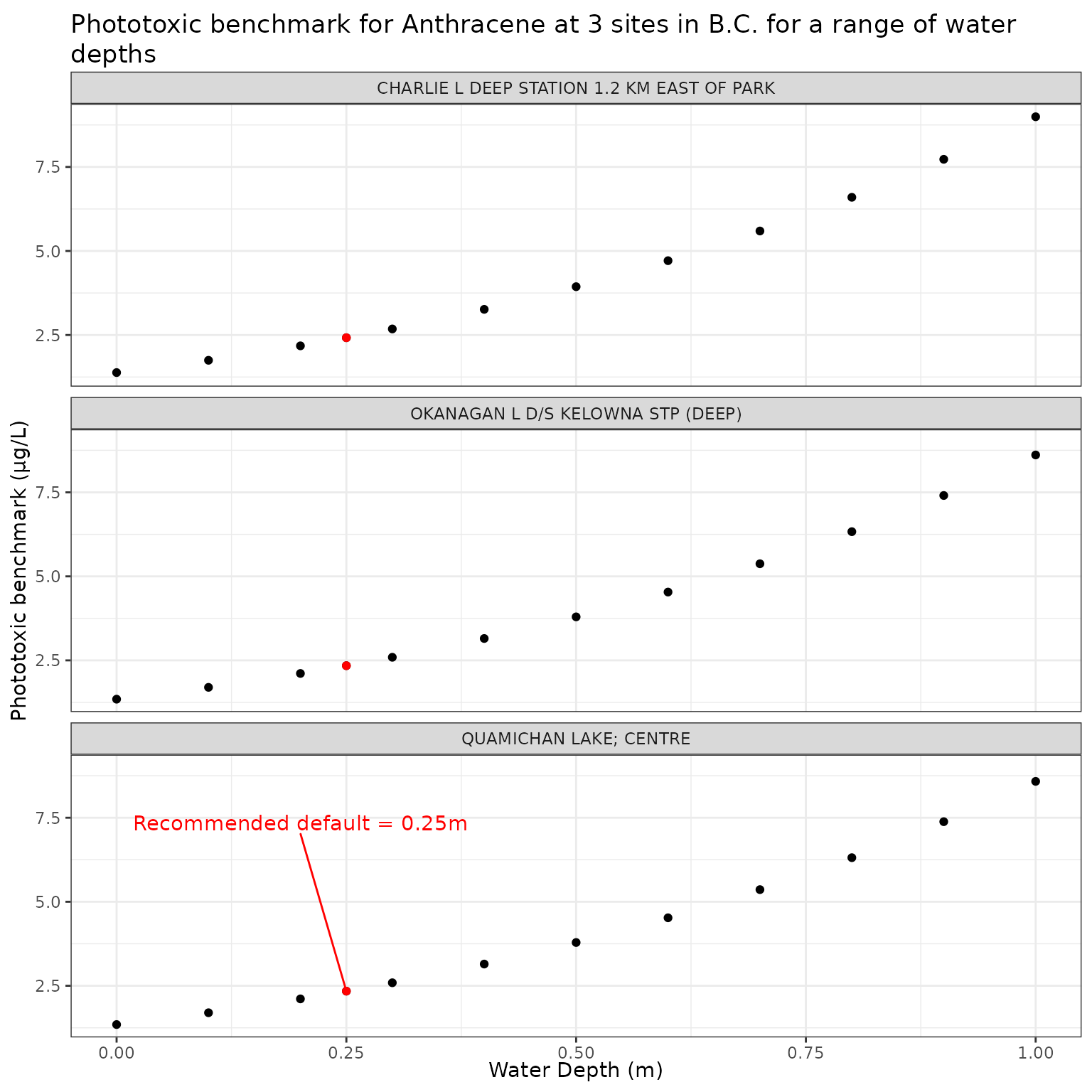
The depth at which the photoxicity of a PAC is determined should be a conservative one - i.e., a depth at which sensitive species/life stages exist and thus would be exposed. The default is set at 0.25m.
We can test the effect of depth on phototoxic benchmark by varying elevation from water level to 1m below the surface:
Effect of varying Water Depth on phototoxic benchmark and ratio of phototoxic:narcotic benchmark for Anthracene
Show/Hide Code
depth_test_a <- multi_pb(
  sites,
  pah = "Anthracene",
  varying = "depth_m",
  vals = depth_vals,
  DOC = 5,
  o3_tc = 300,
  tauaer = 0.235
)

ggplot(depth_test_a, aes(x = depth_m, y = phototoxic_benchmark)) +
  geom_point() +
  geom_point(
    data = filter(depth_test_a, depth_m == 0.25),
    colour = "red"
  ) +
  geom_text_repel(
    data = filter(
      depth_test_a,
      depth_m == 0.25,
      name == "QUAMICHAN LAKE; CENTRE"
    ),
    colour = "red",
    label = "Recommended default = 0.25m",
    nudge_x = -0.05,
    nudge_y = 5
  ) +
  facet_wrap(vars(name), ncol = 1) +
  labs(
    title = "Phototoxic benchmark for Anthracene at 3 sites in B.C. for a range of water depths",
    x = "Water Depth (m)",
    y = "Phototoxic benchmark (μg/L)"
  )
Show/Hide Code
ggplot(depth_test_a, aes(x = depth_m, y = p_n_ratio)) +
geom_point() +
geom_point(
data = filter(depth_test_a, depth_m == 0.25),
colour = "red"
) +
geom_text_repel(
data = filter(
depth_test_a,
depth_m == 0.25,
name == "QUAMICHAN LAKE; CENTRE"
),
colour = "red",
label = "Recommended default = 0.25m",
nudge_x = -0.05,
nudge_y = 0.1
) +
facet_wrap(vars(name), ncol = 1) +
labs(
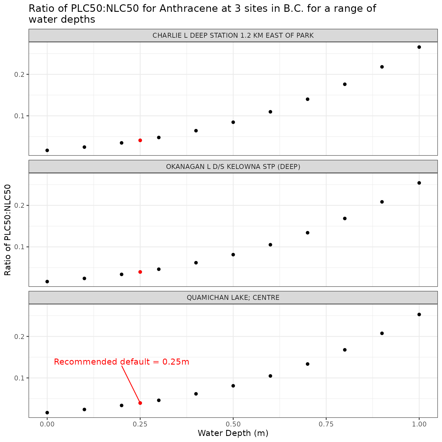
title = "Ratio of phototoxic:narcotic benchmark for Anthracene at 3 sites in B.C. for a range of\nwater depths",
x = "Water Depth (m)",
y = "Ratio of phototoxic:narcotic benchmark"
)
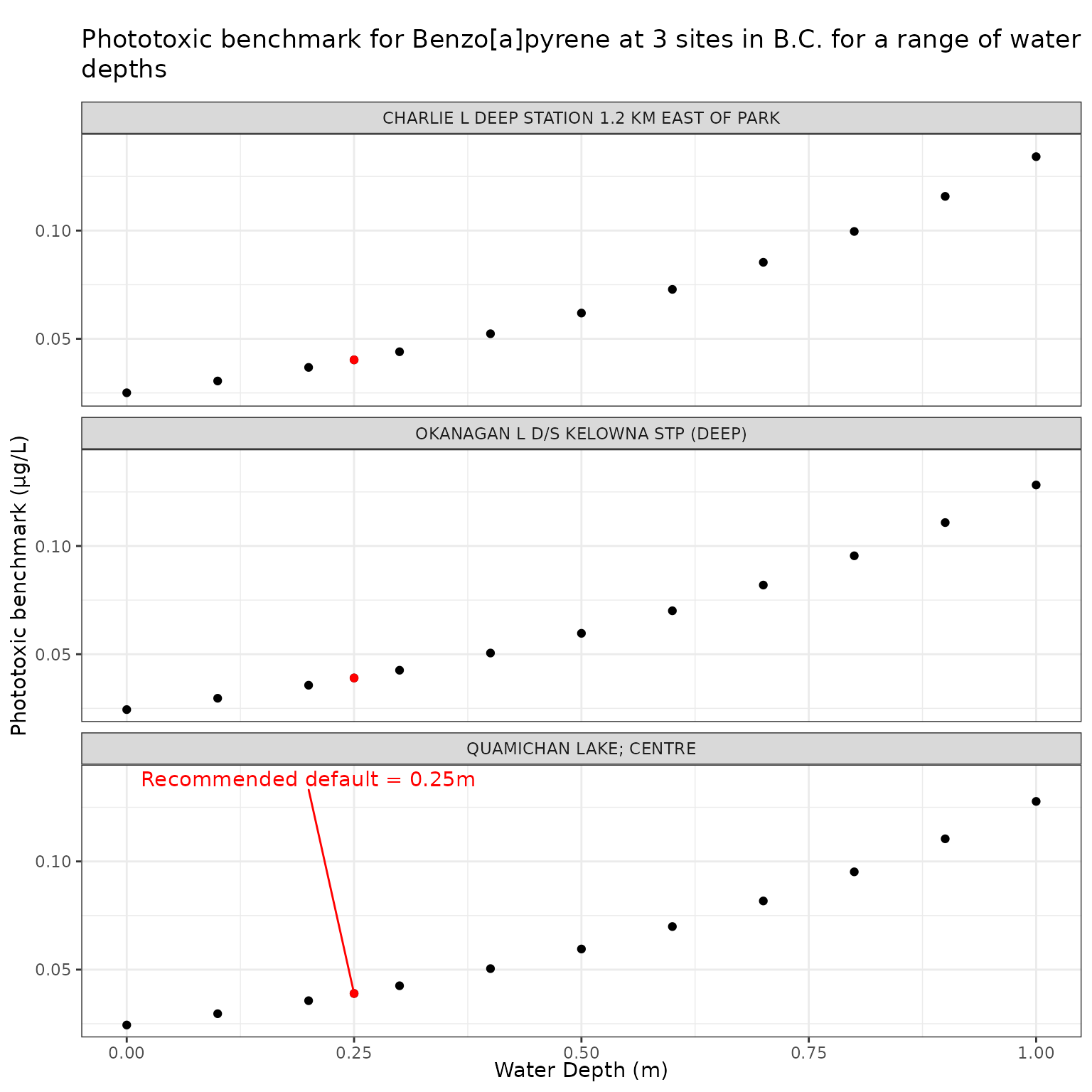
Effect of varying Water Depth on phototoxic benchmark and ratio of phototoxic:narcotic benchmark for Benzo[a]pyrene
Show/Hide Code
depth_test_b <- multi_pb(
  sites,
  pah = "Benzo[a]pyrene",
  varying = "depth_m",
  vals = depth_vals,
  DOC = 5,
  o3_tc = 300,
  tauaer = 0.235
)

ggplot(depth_test_b, aes(x = depth_m, y = phototoxic_benchmark)) +
  geom_point() +
  geom_point(
    data = filter(depth_test_b, depth_m == 0.25),
    colour = "red"
  ) +
  geom_text_repel(
    data = filter(
      depth_test_b,
      depth_m == 0.25,
      name == "QUAMICHAN LAKE; CENTRE"
    ),
    colour = "red",
    label = "Recommended default = 0.25m",
    nudge_x = -0.05,
    nudge_y = 0.1
  ) +
  facet_wrap(vars(name), ncol = 1) +
  labs(
    title = "Phototoxic benchmark for Benzo[a]pyrene at 3 sites in B.C. for a range of water depths",
    x = "Water Depth (m)",
    y = "Phototoxic benchmark (μg/L)"
  )
Show/Hide Code
ggplot(depth_test_b, aes(x = depth_m, y = p_n_ratio)) +
geom_point() +
geom_point(
data = filter(depth_test_b, depth_m == 0.25),
colour = "red"
) +
geom_text_repel(
data = filter(
depth_test_b,
depth_m == 0.25,
name == "QUAMICHAN LAKE; CENTRE"
),
colour = "red",
label = "Recommended default = 0.25m",
nudge_x = -0.05,
nudge_y = 0.05
) +
facet_wrap(vars(name), ncol = 1) +
labs(
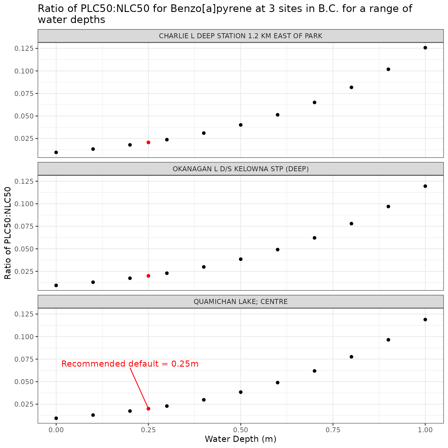
title = "Ratio of phototoxic:narcotic benchmark for Benzo[a]pyrene at 3 sites in B.C. for a range of\nwater depths",
x = "Water Depth (m)",
y = "Ratio of phototoxic:narcotic benchmark"
)
Radiative transfer scheme (nstr)
Number of streams for radiative transfer calculations:
- If
nstr< 2, uses 2-stream delta-Eddington (faster) - if
nstr>= 2, uses n-stream discrete ordinates (more accurate: must be even number, maximum = 32)
Show/Hide Code
out <- multi_pb(
  sites,
  pah = "Anthracene",
  varying = "nstr",
  vals = c(-2, 4),
  DOC = 5,
  o3_tc = 300,
  tauaer = 0.235
) |>
  mutate(nstr = factor(nstr))

ggplot(out, aes(x = name, y = phototoxic_benchmark, colour = nstr)) +
  geom_point() +
  labs(
    title = "Calculated phototoxic benchmark using two different TUV methods for radiative transfer",
    x = "Site"
  ) +
  theme(axis.text.x = element_text(angle = 355))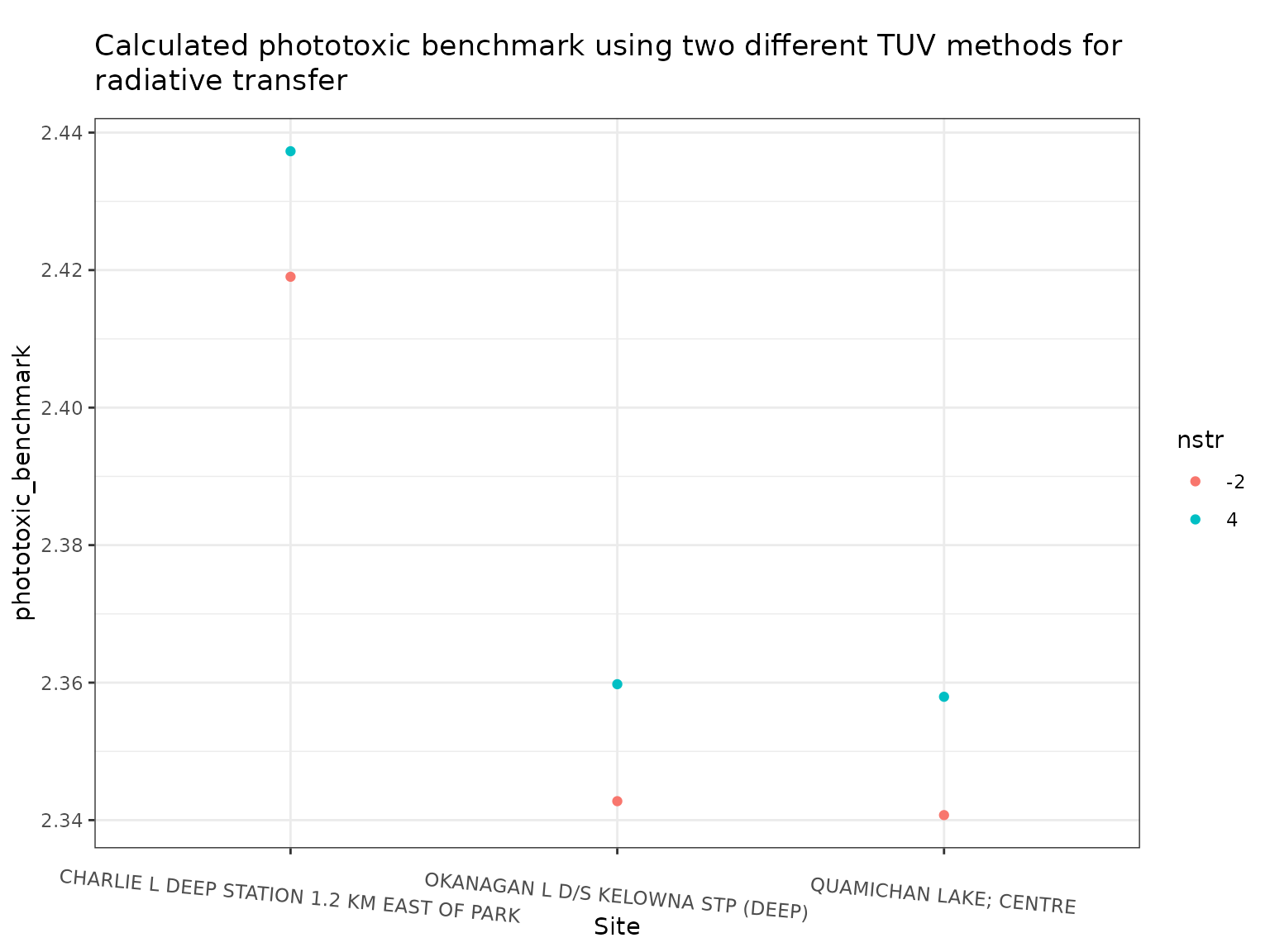
Show/Hide Code
ggplot(out, aes(x = name, y = timing, colour = nstr)) +
  geom_point() +
  labs(
    title = "Execution time of TUV model runs with different methods for radiative transfer",
    x = "Site",
    y = "Execution Time (s)"
  ) +
  theme(axis.text.x = element_text(angle = 355))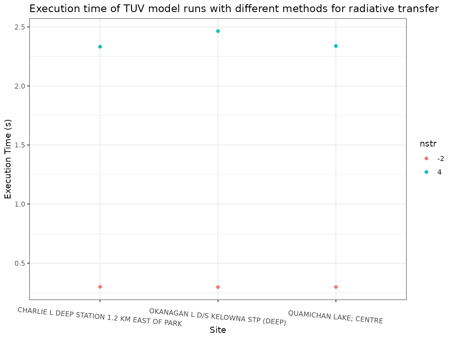
We can see that there are small differences in the calculated
phototoxic benchmark when using different values of nstr,
with the values when calculated using nstr = -2 being on
average 0.73% lower than when using nstr = 4. Using
nstr = 4 however, is about 9 times slower than using
nstr = -2. In most cases, unless high precision is
required, it is likely that using the much faster nstr = -2
should be the default.
Methylated Polycyclic Aromatic Compounds
Absorption spectra for methylated PACs are not all available from published sources, so it would be beneficial to be able to approximate them for calculating water quality guidelines. In this section we will look at the feasibilty of using the absorbance spectra from a methylated PAC’s parent compound as a proxy for the specific spectra. We will do this by calculating the phototoxic benchmark for various methylated PACs for which we have absorbance spectra, and comparing these values to those calculated using the absorbance spectra of the parent PAC.
For these comparisons we will limit it to just one site in the Okanagan.
okanagan <- filter(sites, emsid == "0500236")Show/Hide Code
# Define some functions:
ma_plot <- function(chemicals) {
  pahwq:::molar_absorption |>
    filter(chemical %in% tolower(chemicals)) |>
    mutate(
      chemical = factor(chemical, levels = tolower(chemicals))
    ) |>
    ggplot(aes(x = wavelength, y = molar_absorption, colour = chemical)) +
    geom_point() +
    labs(
      title = paste0(
        "Molar absorption of ",
        chemicals[1],
        " and methylated derivatives"
      ),
      y = "Molar absorption (L/mol/cm)"
    )
}

nb_plot <- function(chemicals) {
  pahwq:::nlc50_lookup |>
    filter(chemical %in% tolower(chemicals)) |>
    mutate(
      narcotic_benchmark = vapply(chemical, narcotic_benchmark, FUN.VALUE = 1),
      chemical = factor(chemical, levels = tolower(chemicals))
    ) |>
    ggplot(aes(x = log_kow, y = narcotic_benchmark, colour = chemical)) +
    geom_point() +
    labs(
      title = paste0(
        "Narcotic benchmark of ",
        chemicals[1],
        " and its methylated derivatives"
      ),
      y = "Narcotic benchmark (ug/L)"
    )
}

pb_surrogates <- function(chemicals) {
  multi_pb(
    okanagan,
    site = "name",
    pah = chemicals,
    varying = "Kd_ref",
    vals = c(1, 150),
    depth_m = 0.25
  ) |>
    group_by(Kd_ref) |>
    rowwise() |>
    mutate(
      Pabs_parent = p_abs(tuv_res, tolower(chemicals[1])),
      pb_parent = phototoxic_benchmark(Pabs_parent, PAC)
    ) |>
    ungroup() |>
    mutate(
      PAC = factor(PAC, levels = chemicals)
    ) |>
    pivot_longer(
      cols = c(phototoxic_benchmark, pb_parent),
      names_to = "abs_spectra",
      values_to = "phototoxic_benchmark"
    ) |>
    mutate(
      p_n_ratio = phototoxic_benchmark / narcotic_benchmark,
      abs_spectra = case_when(
        abs_spectra == "phototoxic_benchmark" ~ "specific",
        abs_spectra == "pb_parent" ~ "parent"
      )
    )
}

pb_plot <- function(df) {
  ggplot(df, aes(x = PAC, y = phototoxic_benchmark, colour = abs_spectra)) +
    geom_point() +
    facet_wrap(
      vars(Kd_ref),
      ncol = 1,
      scales = "free_y",
      labeller = as_labeller(function(x) paste0("Kd(305) = ", x))
    ) +
    geom_text_repel(
      data = filter(df, PAC != chemicals[1]),
      mapping = aes(label = round(p_n_ratio, 3)),
      show.legend = FALSE
    ) +
    labs(
      title = paste0(
        "Comparison of phototoxic benchmark of methylated ",
        chemicals[1],
        ", using\nspecific absorption spectra vs absorption spectra of parent compound"
      ),
      y = "Phototoxic benchmark (ug/L)",
      colour = "Absorption spectra used",
      caption = "*Text labels indicate the ratio of phototoxic:narcotic benchmark"
    )
}
Napthalene
To start, we can examine the molar absorption specra of three methylated Naphthalene derivatives, as compared to unmethylated Naphthalene:
Show/Hide Code
chemicals <- c(
  "Naphthalene",
  "1-Methylnaphthalene",
  "2,6-Dimethylnaphthalene",
  "1,6,7-Trimethylnaphthalene"
)

ma_plot(chemicals)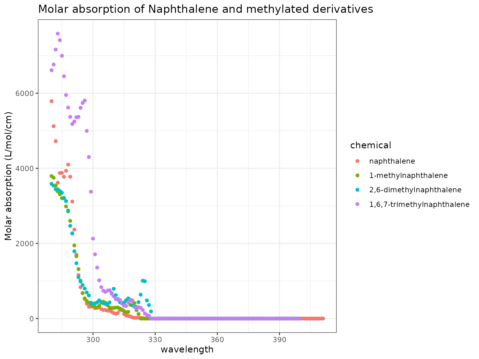
We can see in general that more highly methylated compounds have greater absorption, though it is not consistent across the spectrum.
We can also examine the properties and narcotic toxicity of Naphthalene and its methylated variants:
Show/Hide Code
nb_plot(chemicals)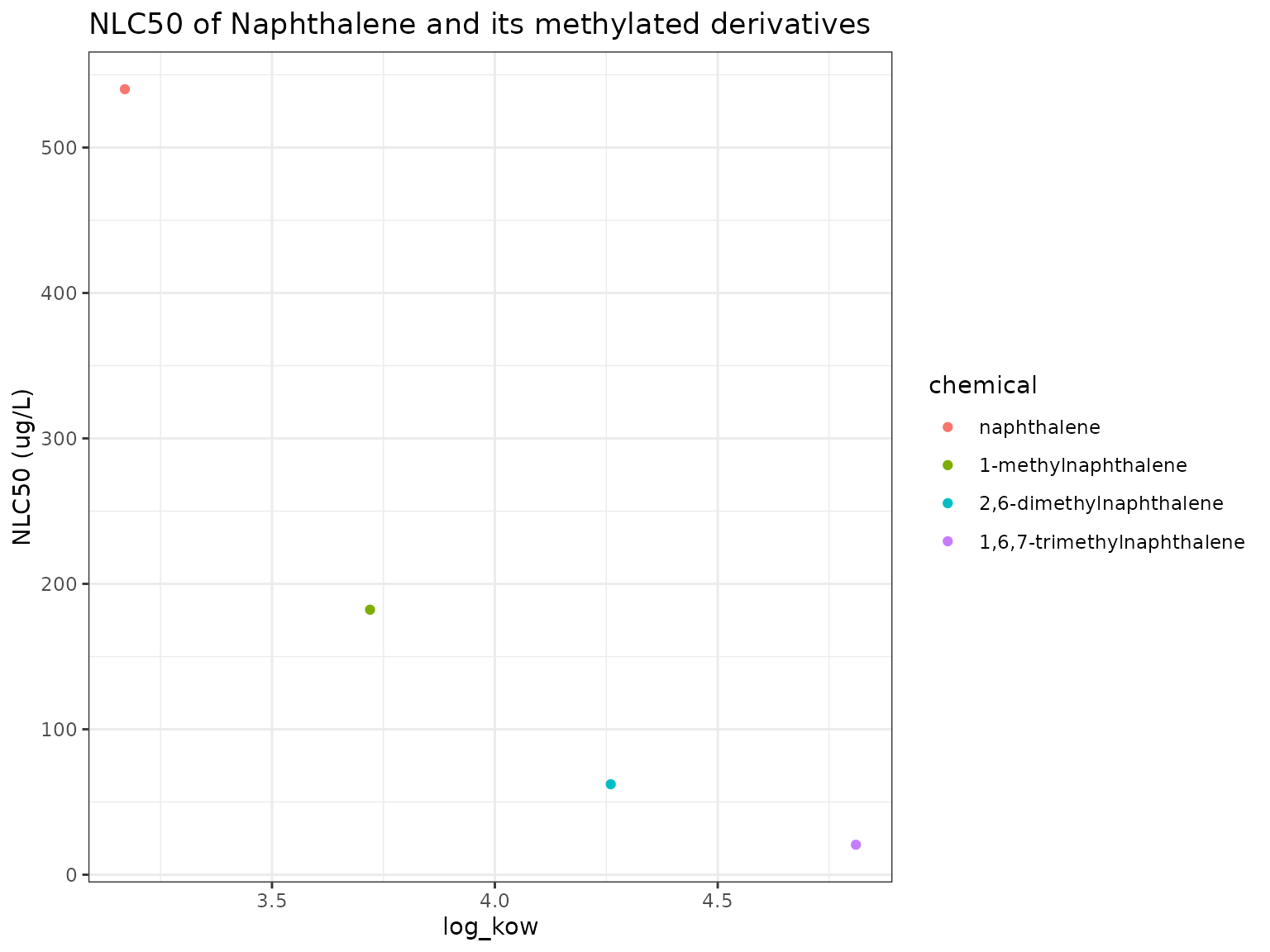
We can see here that 1,6,7-Trimethylnaphthalene has the highest log(KoW) and lowest narcotic benchmark.
Finally, we can compare the phototoxicity (phototoxic benchmark) of Naphthalene and its methylated derivatives at the Okanagan site, at the two values of (1 and 150).
Show/Hide Code
df <- pb_surrogates(chemicals)
pb_plot(df) +
  theme(axis.text.x = element_text(angle = 355))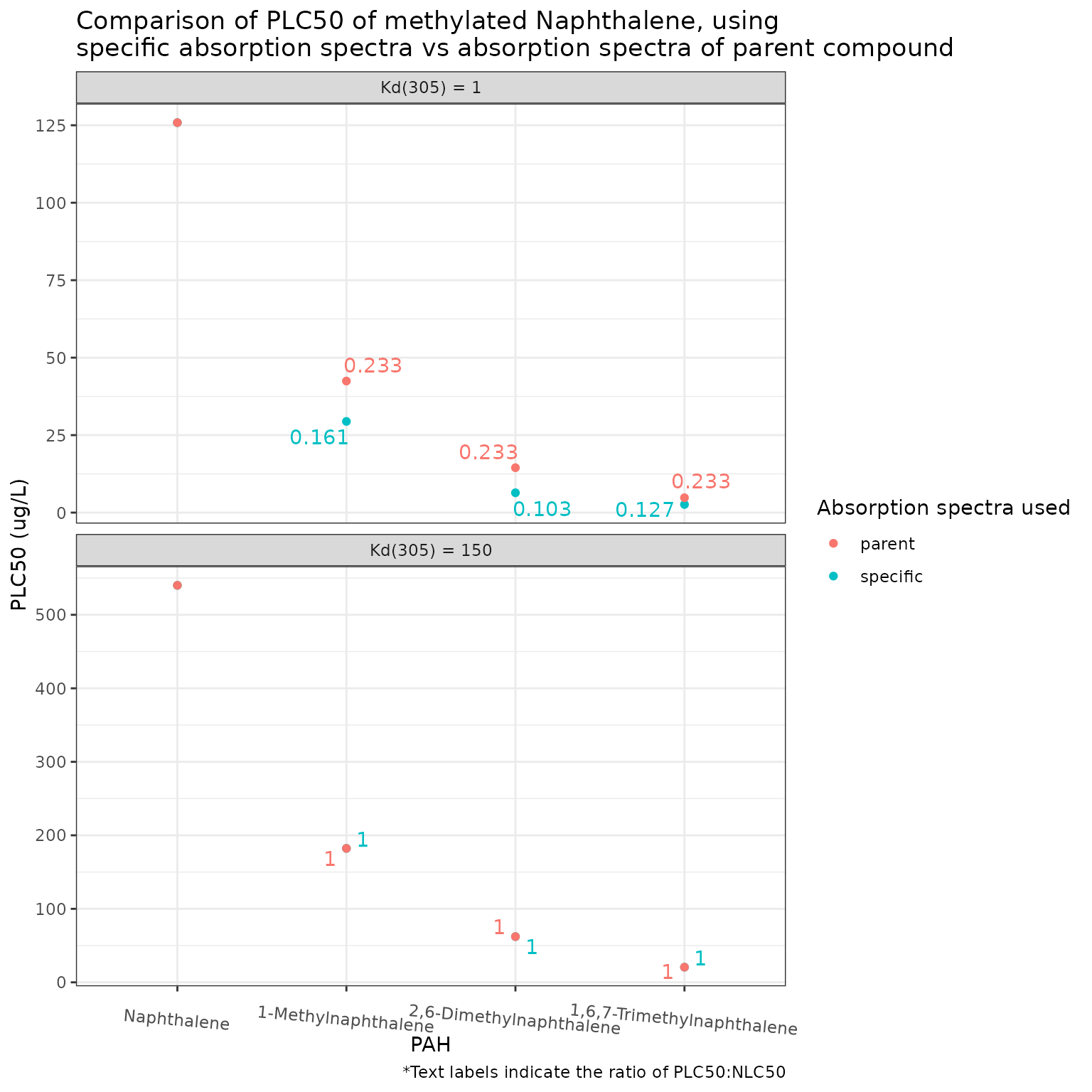
Here we can see that a lower phototoxic benchmark (higher phototoxicity) is calculated for all methylated naphthalenes when the absorption spectra of the methylated compound is used, as compared to when that of the parent compound (Naphthalene) is used. This difference is much greater when there is higher light penetration (lower Kd) - which is to be expected, as when there is less light penetration the phototoxic benchmark approaches the narcotic benchmark so the absorption spectra of the chemical becomes irrelevant.
Phenanthrene
As above, we can visualize the absorption spectra of Phenanthrene and 9-Methylphenanthrene:
Show/Hide Code
chemicals <- c("Phenanthrene", "9-Methylphenanthrene")

ma_plot(chemicals)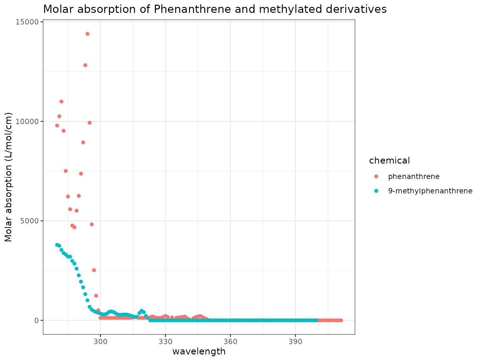
Here we see that the parent compound Phenanthrene has much higher absorption than 9-Methylphenanthrene at the low end of the light spectrum.
Show/Hide Code
nb_plot(chemicals)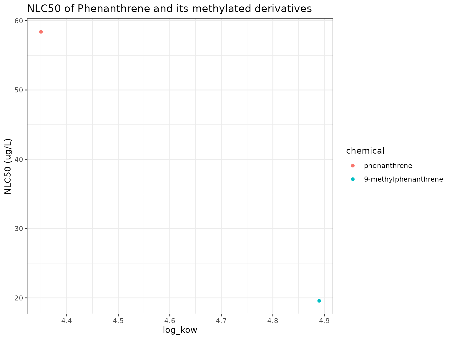
9-Methylphenanthrene has higher narcotic toxicity (lower narcotic benchmark) than its parent Phenanthrene.
Show/Hide Code
phototoxic_benchark_df_phenanthrene <- pb_surrogates(chemicals)
pb_plot(phototoxic_benchark_df_phenanthrene)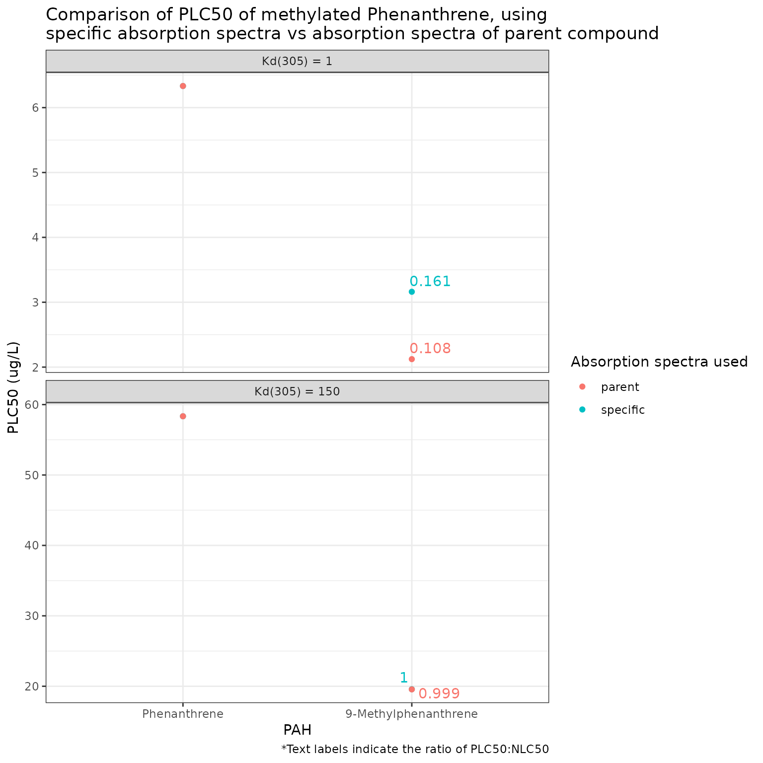
Using the parent molar absorption spectra for 9-Methylphenanthrene gives a more conservative phototoxic benchmark than using the specific spectra for the methylated compound. This is different than the case for Naphthalene.
Similar to Naphthalene, this only appears to be substantially different at high light penetration (low Kd(305)).
Anthracene
As above, we can visualize the absorption spectra of Anthracene and 9-Methylanthracene:
Show/Hide Code
chemicals <- c("Anthracene", "9-Methylanthracene")
ma_plot(chemicals)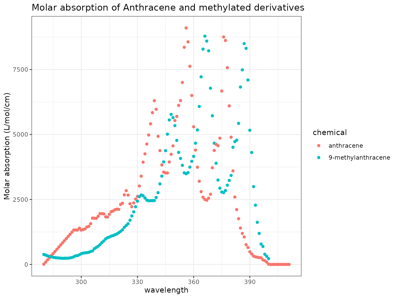
The absorption spectra for both Anthracene and 9-Methylanthracene is very broad compared to that of the other PAC compounds.
Show/Hide Code
nb_plot(chemicals)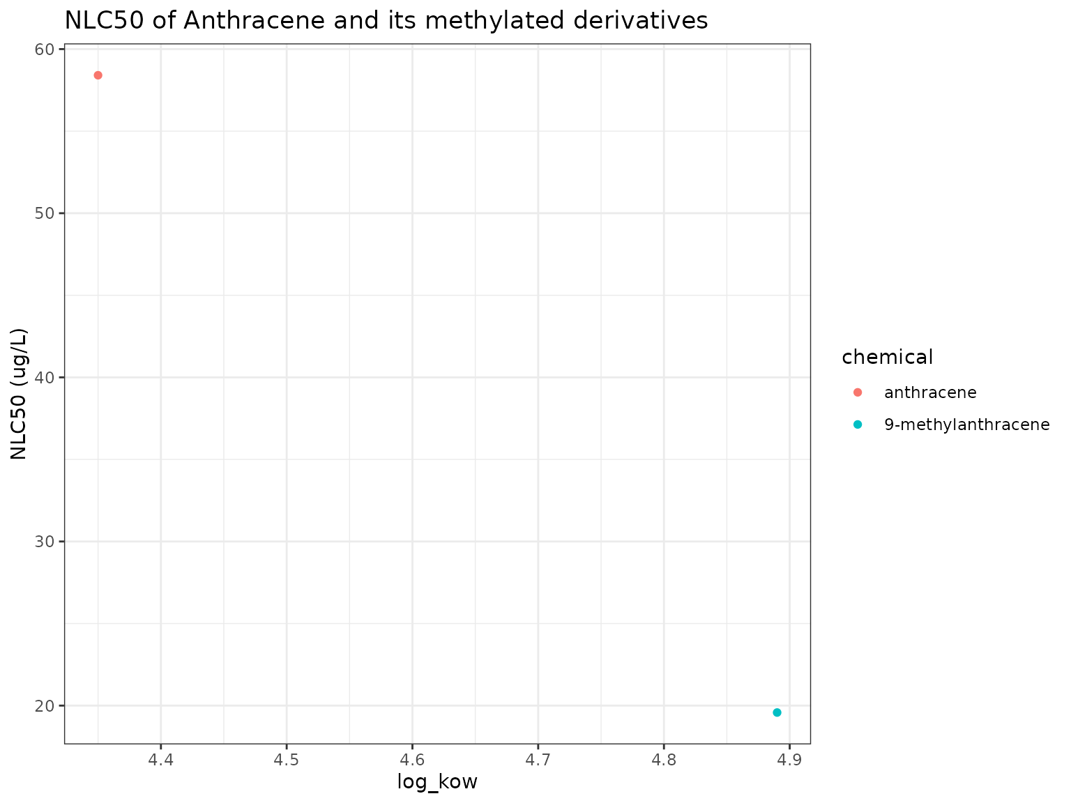
9-Methylanthracene has higher narcotic toxicity (lower narcotic benchmark) than its parent Anthracene.
Show/Hide Code
phototoxic_benchmark_df_anthracene <- pb_surrogates(chemicals)
pb_plot(phototoxic_benchmark_df_anthracene) +
  theme(axis.text.x = element_text(angle = 355))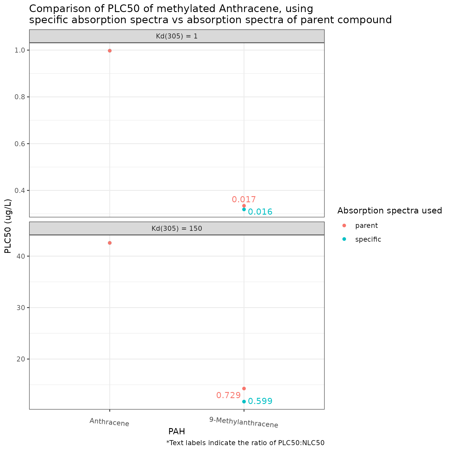
Using the parent absorption spectra for 9-Methylanthracene results in a less conservative phototoxic benchmark than if the specific absorption spectra is used. Contrary to that seen in the other PACs above, this effect is still quite pronounced at high light attenuation (Kd(305) = 150), presumably because of the broad absorption spectra exhibited by both Anthracene and 9-Methylanthracene.
Pyrene
Show/Hide Code
chemicals <- c("Pyrene", "1-Methylpyrene")

ma_plot(chemicals)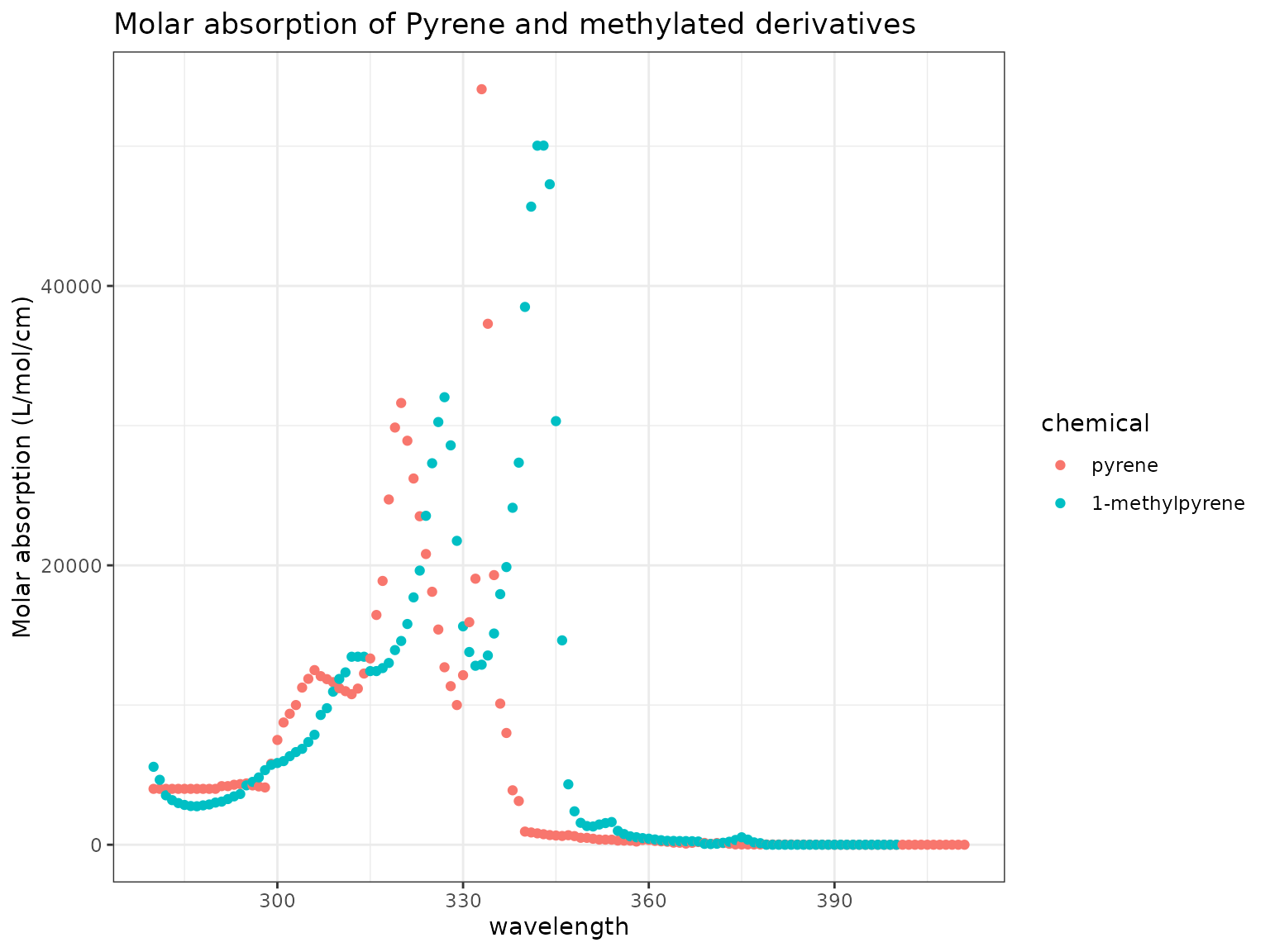
Show/Hide Code
nb_plot(chemicals)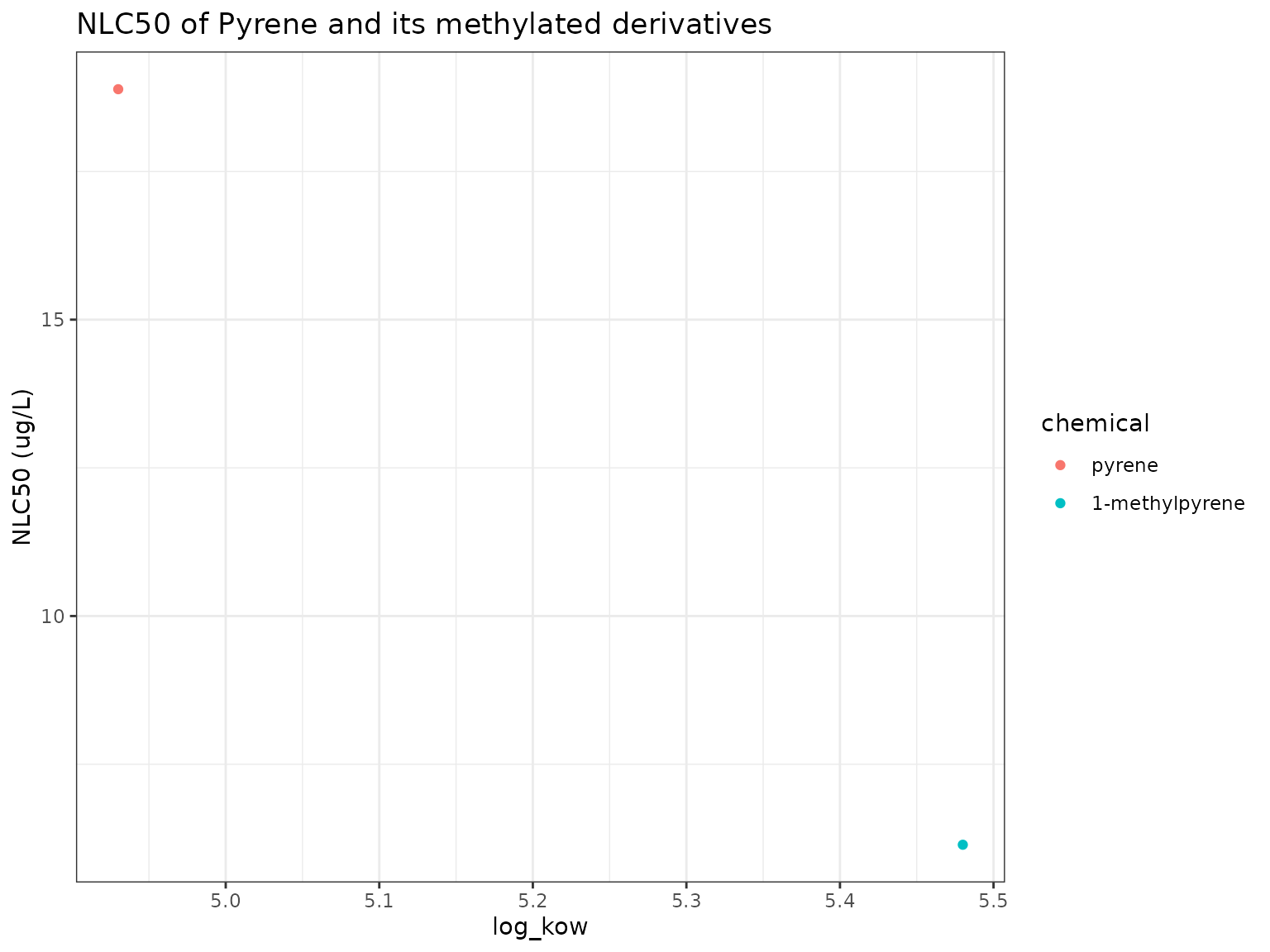
9-Methylpyrene has higher narcotic toxicity (lower narcotic benchmark) than its parent Pyrene.
Show/Hide Code
phototoxic_benchmark_df_pyrene <- pb_surrogates(chemicals)
pb_plot(phototoxic_benchmark_df_pyrene)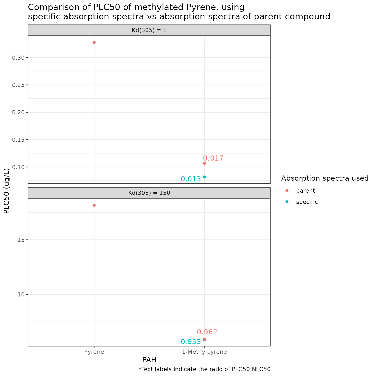
Using the parent absorption spectra for 9-Methylpyrene results in a less conservative phototoxic benchmark than if the specific absorption spectra is used.
Chrysene
Show/Hide Code
chemicals <- c("Chrysene", "1-Methylchrysene")
ma_plot(chemicals)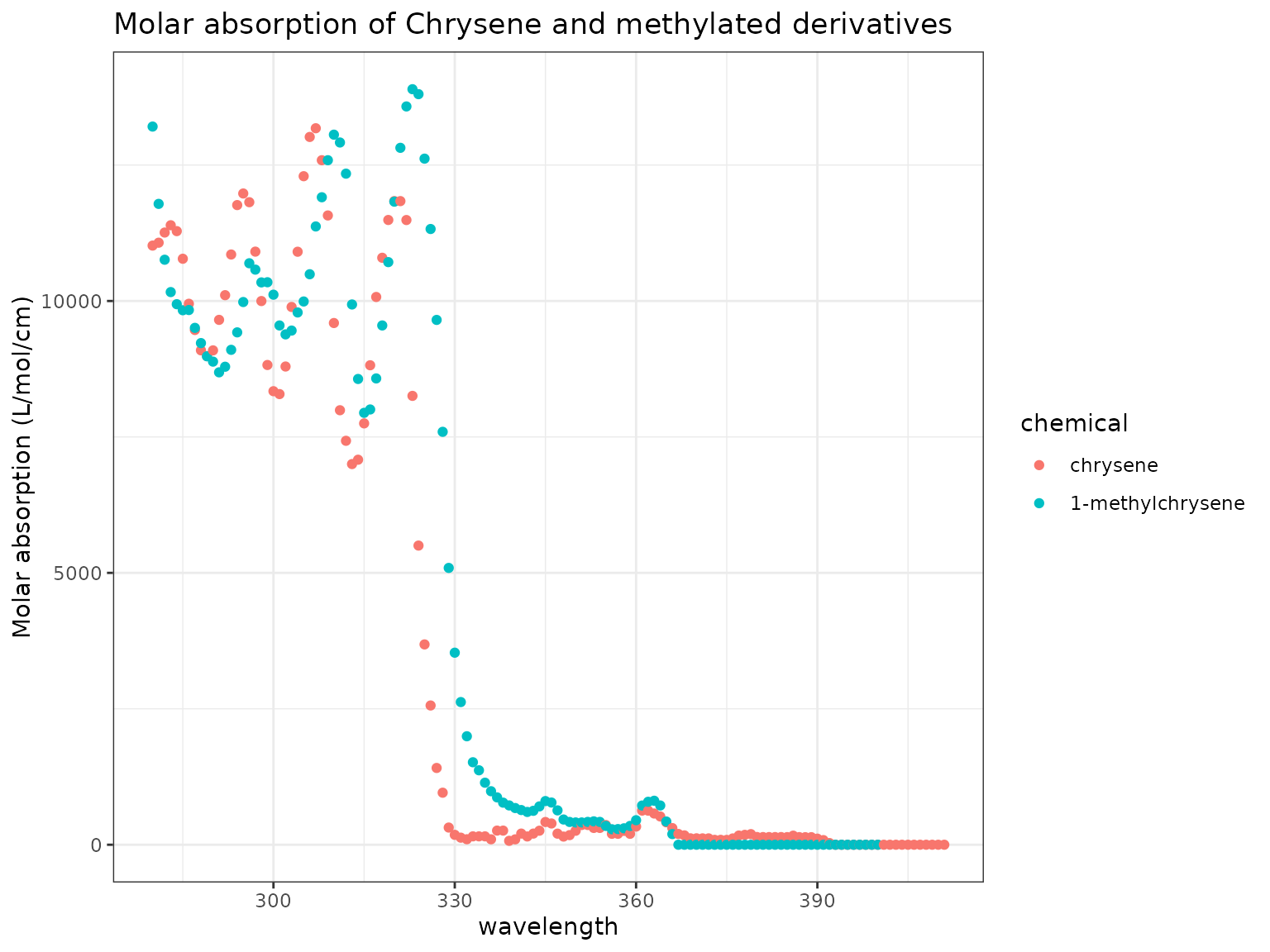
Show/Hide Code
nb_plot(chemicals)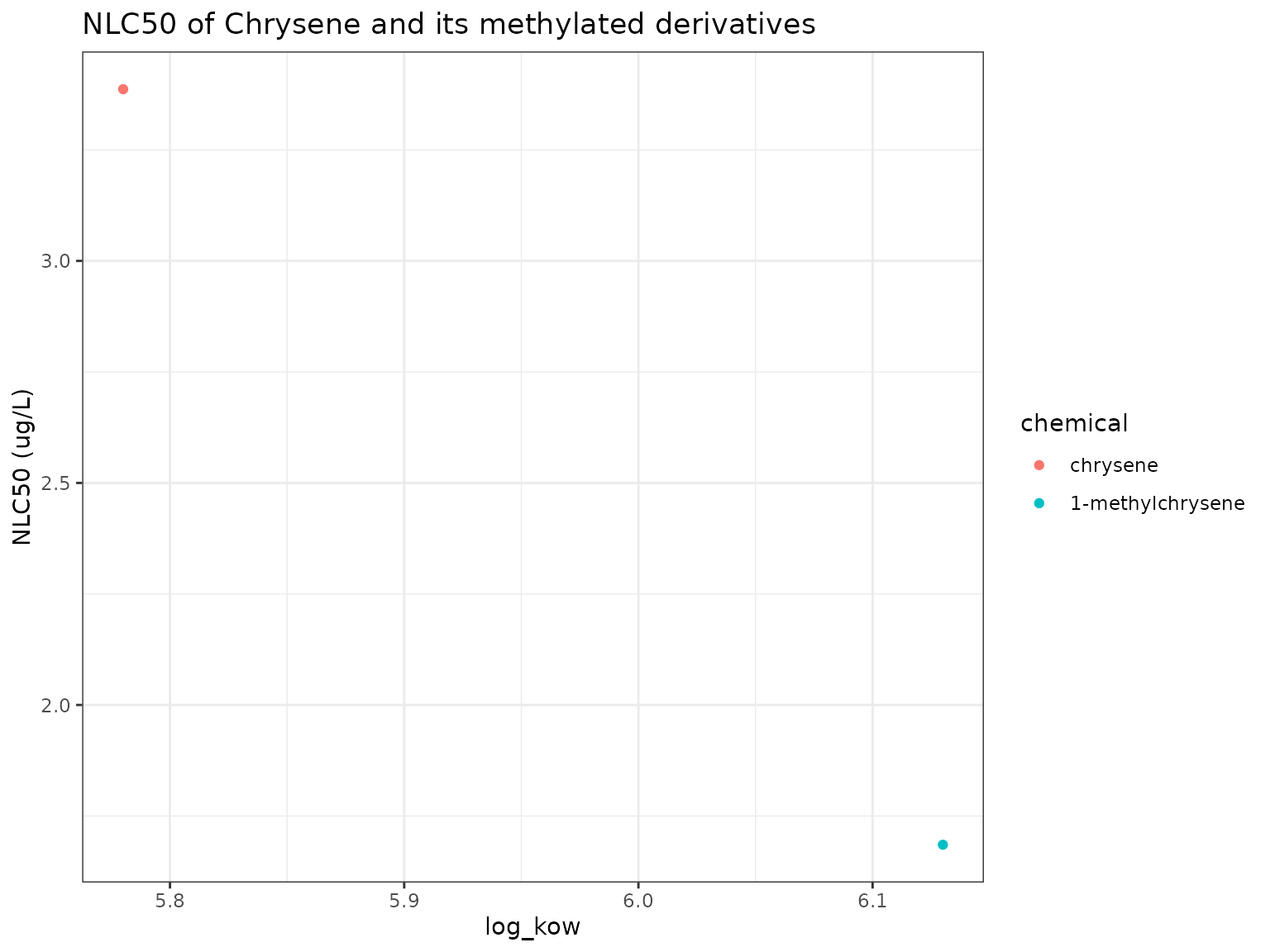
Similar to the other methylated PACs, 1-Methylchrysene has a lower narcotic benchmark (higher narcotic toxicity) than its parent Chrysene.
Show/Hide Code
phototoxic_benchmark_df_chrysene <- pb_surrogates(chemicals)
pb_plot(phototoxic_benchmark_df_chrysene)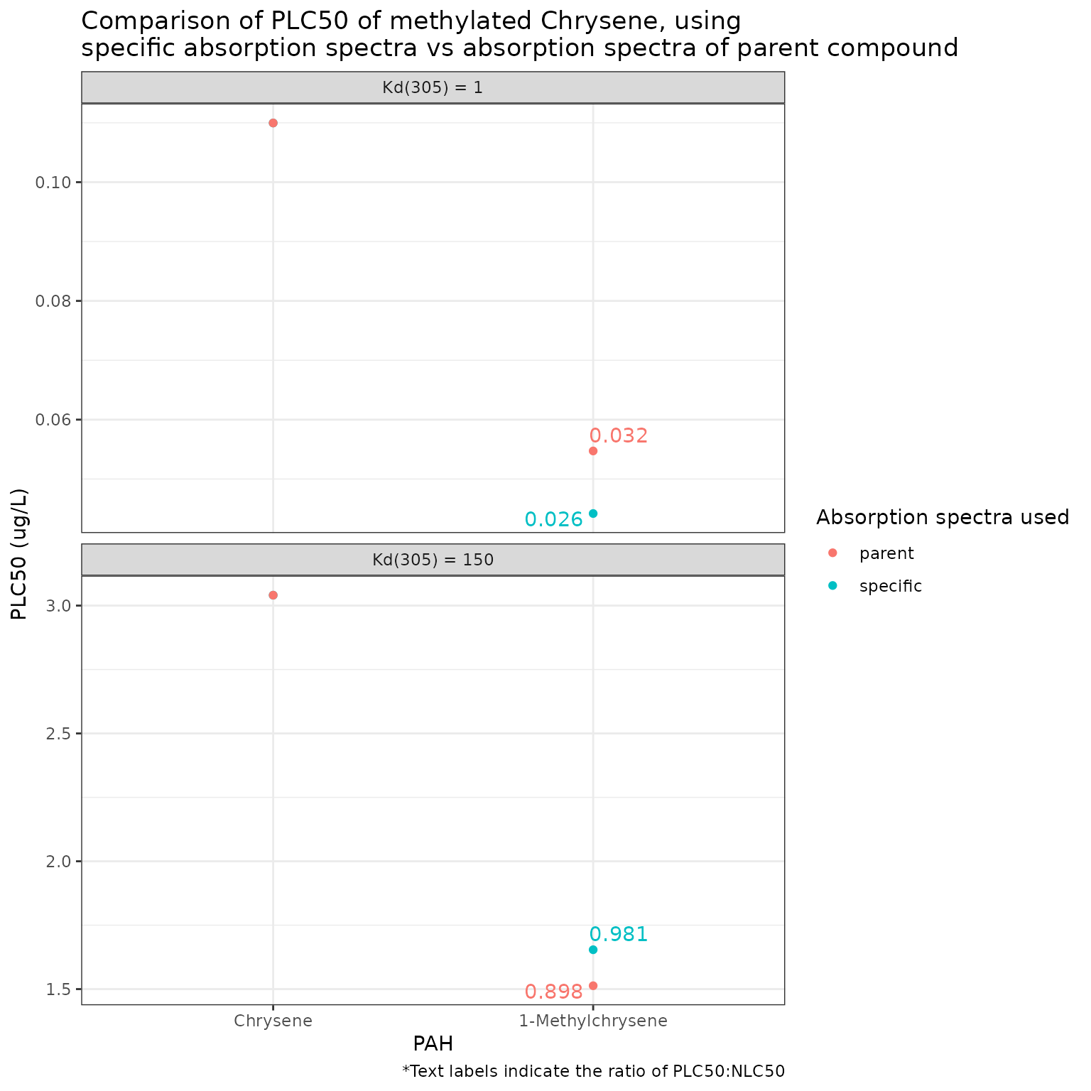
The results for Chrysene and 1-Methylchrysene show that the effect of using the absorbance spectra of a parent compound can be different depending on the light intensity/attenuation. At low light attenuation (Kd(305) = 1), the specific spectra gives a more conservative phototoxic benchmark for 1-Methylchrysene than that obtained using the spectra from Chrysene, while the opposite is true at high light attenuation (Kd(305) = 100).
These results show that substituting the absorption spectra of a parent compound when that of a specific methylated PAC is unknown is possible, but also somewhat complicated. Differences in absorption spectra between methylated PACs and that of their parent was quite variable across compounds. The difference in the resulting calculated phototoxic benchmark is generally quite small and thus it is likely reasonable to use the absorption spectra of a parent when it is not available for a methylated PAC. However, the magnitude and even the sign of the difference is highly variable. In all cases examined, the narcotic benchmark of the methylated compounds was lower than that of the parent compounds (i.e., they are more toxic), however the final phototoxicity (phototoxic benchmark) depended on the differences in the absorption spectra and, in some cases, the level of light attenuation.