Get Started with fasstr

fasstr, the Flow Analysis Summary Statistics Tool for R, is a set of R functions to tidy, summarize, analyze, trend, and visualize streamflow data. This package summarizes continuous daily mean streamflow data into various daily, monthly, annual, and long-term statistics, completes trending and frequency analyses, with outputs in both table and plot formats.

Features

This package provides functions for streamflow data analysis, including:

• data tidying (to prepare data for analyses; add_* and fill_* functions),
• data screening (to identify data range, outliers and missing data; screen_* functions),
• calculating summary statistics (long-term, annual, monthly and daily statistics; calc_*functions),
• computing analyses (volume frequency analyses and annual trending; compute_* functions), and,
• visualizing data (plotting the various statistics; plot_* functions).

Useful features of functions include:

• the integration of the tidyhydat package to pull streamflow data from a Water Survey of Canada HYDAT database for analyses;
• arguments for filtering of years and months in analyses and plotting;
• choosing the start month of your water year;
• selecting for rolling day averages (e.g. 7-day rolling average); and,
• choosing how missing dates are handled, amongst others.

This package is maintained by the Water Protection and Sustainability Branch of the British Columbia Land, Water and Resource Stewardship.

Installation

You can install fasstr directly from CRAN:

install.packages("fasstr")

To install the development version from GitHub, use the remotes package then the fasstr package:

if(!requireNamespace("remotes")) install.packages("remotes")
remotes::install_github("bcgov/fasstr")

Several other packages will be installed with fasstr. These include tidyhydat for downloading Water Survey of Canada hydrometric data, zyp for trending, ggplot2 for creating plots, and tidyr and dplyr for data wrangling and summarizing, amongst others.

To use the station_number argument and pull data directly from a Water Survey of Canada HYDAT database into fasstr functions, download a HYDAT file using the following code:

tidyhydat::download_hydat()

Using fasstr

There are several vignettes to provide more information on the usage of fasstr functions and how to customize them with various argument options.

• Get Started with fasstr
• fasstr Users Guide
• Computing an Annual Trends Analysis
• Computing a Volume Frequency Analysis
• Computing a Full fasstr Analysis
• fasstr Internal Workflows

Data Input

All functions in fasstr require a daily mean streamflow data set from one or more hydrometric stations. Long-term and continuous data sets are preferred for most analyses, but seasonal and partial data can be used. Other daily time series data, like temperature, precipitation or water levels, may also be used, but with certain caution as some calculations/conversions are based on units of streamflow (cubic metres per second). Data is provided to each function using the either the data argument as a data frame of flow values, or the station_number argument as a list of Water Survey of Canada HYDAT station numbers.

When using the data option, a data frame of daily data containing columns of dates (YYYY-MM-DD in date format), values (mean daily discharge in cubic metres per second in numeric format), and, optionally, grouping identifiers (character string of station names or numbers) is called. By default the functions will look for columns identified as ‘Date’, ‘Value’, and ‘STATION_NUMBER’, respectively, to be compatible with the ‘tidyhydat’ defaults, but columns of different names can be identified using the dates, values, groups column arguments (ex. values = Yield_mm). The following is an example of an appropriate data frame (STATION_NUMBER not required):

##   STATION_NUMBER       Date Value
## 1        08NM116 1949-04-01  1.13
## 2        08NM116 1949-04-02  1.53
## 3        08NM116 1949-04-03  2.07
## 4        08NM116 1949-04-04  2.07
## 5        08NM116 1949-04-05  2.21
## 6        08NM116 1949-04-06  2.21

Alternatively, you can directly pull a flow data set directly from a HYDAT database (if installed) by providing a list of station numbers in the station_number argument (ex. station_number = "08NM116" or station_number = c("08NM116", "08NM242")) while leaving the data arguments blank. A data frame of daily streamflow data for all stations listed will be extracted using tidyhydat and then fasstr calculations will produce results of the functions.

This package allows for multiple stations (or other groupings) to be analyzed in many of the functions provided identifiers are provided using the groups column argument (defaults to STATION_NUMBER). If grouping column doesn’t exist or is improperly named, then all values listed in the values column will be summarized.

Function Types

Tidying

These functions, start with either add_* or fill_*, add columns and rows, respectively, to streamflow data frames to help set up your data for further analysis. Examples include adding rolling means, adding date variables (WaterYear, Month, DayofYear, etc.), adding basin areas, adding columns of volumetric discharge and water yield, and filling dates with missing flow values with NA.

Analysis

The analysis functions summarize your discharge values into various statistics. screen_* functions summarize annual data for outliers and missing dates. calc_* functions calculate daily, monthly, annual, and long-term statistics (e.g. mean, median, maximum, minimum, percentiles, amongst others) of daily, rolling days, and cumulative flow data. compute_* functions also analyze data but produce more in-depth analyses, like frequency and trending analysis, and may produce multiple plots and tables as a result. All tables are in tibble data frame formats. Can use write_flow_data() or write_results() to customize saving tibbles to a local drive.

Visualization

The visualization functions, which begin with plot_*, plot the various summary statistics and analyses as a way to visualize the data. While most plotting function statistics can be customized, some come pre-set with statistics that cannot be changed. Plots can be further modified by the user using the ggplot2 package and its functions. All plots functions produce lists of plots (even if just one produced). Can use write_plots() to customize saving the lists of plots to a local drive (within folders or PDF documents).

Function Options

Daily Rolling Means

If certain n-day rolling mean statistics are desired to be analyzed (e.g. 3- or 7-day rolling means) some functions provide the ability to select for that as function arguments (e.g. rolling_days = 7 and rolling_align = "right"). The rolling day align is the placement of the date amongst the n-day means, where “right” averages the day-of and previous n-1 days, “centre” date is in the middle of the averages, and “left” averages the day-of and the following n-1 days. For your own analyses you can add rolling means to your data set using the add_rolling_means() function.

Year and Month Filtering

To customize your analyses for specific time periods, you can designate the start and end years of your analysis using the start_year and end_year arguments and remove any unwanted years (for partial data sets for example) by listing them in the excluded_years argument (e.g. excluded_years = c(1990, 1992:1994)). Alternatively, some functions have an argument called complete_years that summarizes data from just those years which have complete flow records. Some functions will also allow you to select the months of a year to analyze, using the months argument, as opposed to all months (if you want just summer low-flows, for example). Leaving these arguments blank will result in the summary/analysis of all years and months of the provided data set.

To group analyses by water, or hydrologic, years instead of calendar years, if desired, you can set water_year_start within most functions to another month than 1 (for January). A water year can be defined as a 12-month period that comprises a complete hydrologic cycle (wet seasons can typically cross calendar year), typically starting with the month with minimum flows (the start of a new water recharge cycle). If another start month is desired, you can choose it using the water_year_start argument (numeric month). The water year identifier is designated by the year it ends in (e.g. a water year from Oct 1, 1999 to Sep 30, 2000 is designated as 2000). Start, end and excluded years will be based on the specified water year.

For your own analyses, you can add date variables to your data set using the add_date_variables() or add_seasons() functions.

Drainage Basin Area

Water yield statistics (in millimetres) calculated in the some of the functions require an upstream drainage basin area (in sq. km) using the basin_area argument. If no basin areas are supplied, all yield results will be NA. To apply a basin area (10 sqkm for example) to all daily observations, set the argument as basin_area = 10. If there are multiple stations or groups to apply multiple basin areas (using the groups argument), set them individually using this option: basin_area = c("08NM116" = 795, "08NM242" = 22). If a STATION_NUMBER column exists with HYDAT station numbers, the function will automatically use the basin areas provided in HYDAT, if available, so basin_area is not required. For your own analyses, you can add basin areas to your data set using the add_basin_area() function.

Handling Missing Dates

With the use of the ignore_missing argument in most functions, you can decide how to handle dates with missing flow values in calculations. When you set ignore_missing = TRUE a statistic will be calculated for a given year, all years, or month regardless of if there are missing flow values. When ignore_missing = FALSE the returned value for the period will be NA if there are missing values. To allow some missing dates and still calculate statistics, some functions also including the allowed_missing argument where you provide a percentage (0 to 100) of missing days per time period.

Some functions have an argument called complete_years which can be used, when set to TRUE, to filter out years that have partial data sets (for seasonal or other reasons) and only years with full data are used to calculate statistics.

Examples

Summary statistics example: long-term statistics

To determine the long-term summary statistics of daily data for each month (mean, median, maximum, minimum, and some percentiles) you can use the calc_longterm_daily_stats() function. If the ‘Mission Creek near East Kelowna’ hydrometric station is of interest you can list the station number in the station_number argument to obtain the data (if tidyhydat and HYDAT are installed). Statistics over several months can also be calculated, if of interest. See the summer statistics (from July to September) in this example.

calc_longterm_daily_stats(station_number = "08NM116", 
                          start_year = 1981, 
                          end_year = 2010,
                          custom_months = 7:9, 
                          custom_months_label = "Summer")

## # A tibble: 14 × 8
##    STATION_NUMBER Month      Mean Median Maximum Minimum   P10   P90
##    <chr>          <fct>     <dbl>  <dbl>   <dbl>   <dbl> <dbl> <dbl>
##  1 08NM116        Jan        1.22  1        9.5    0.160 0.540  1.85
##  2 08NM116        Feb        1.16  0.970    4.41   0.140 0.474  1.99
##  3 08NM116        Mar        1.85  1.40     9.86   0.380 0.705  3.80
##  4 08NM116        Apr        8.32  6.26    37.9    0.505 1.63  17.5 
##  5 08NM116        May       23.6  20.8     74.4    3.83  9.33  41.2 
##  6 08NM116        Jun       21.5  19.5     84.5    0.450 6.10  38.9 
##  7 08NM116        Jul        6.48  3.90    54.5    0.332 1.02  15   
##  8 08NM116        Aug        2.13  1.57    13.3    0.427 0.775  4.29
##  9 08NM116        Sep        2.19  1.58    14.6    0.364 0.735  4.35
## 10 08NM116        Oct        2.10  1.60    15.2    0.267 0.794  3.98
## 11 08NM116        Nov        2.04  1.73    11.7    0.260 0.560  3.90
## 12 08NM116        Dec        1.30  1.05     7.30   0.342 0.5    2.33
## 13 08NM116        Long-term  6.17  1.89    84.5    0.140 0.680 19.3 
## 14 08NM116        Summer     3.61  1.98    54.5    0.332 0.799  7.64

Plotting example: daily summary statistics

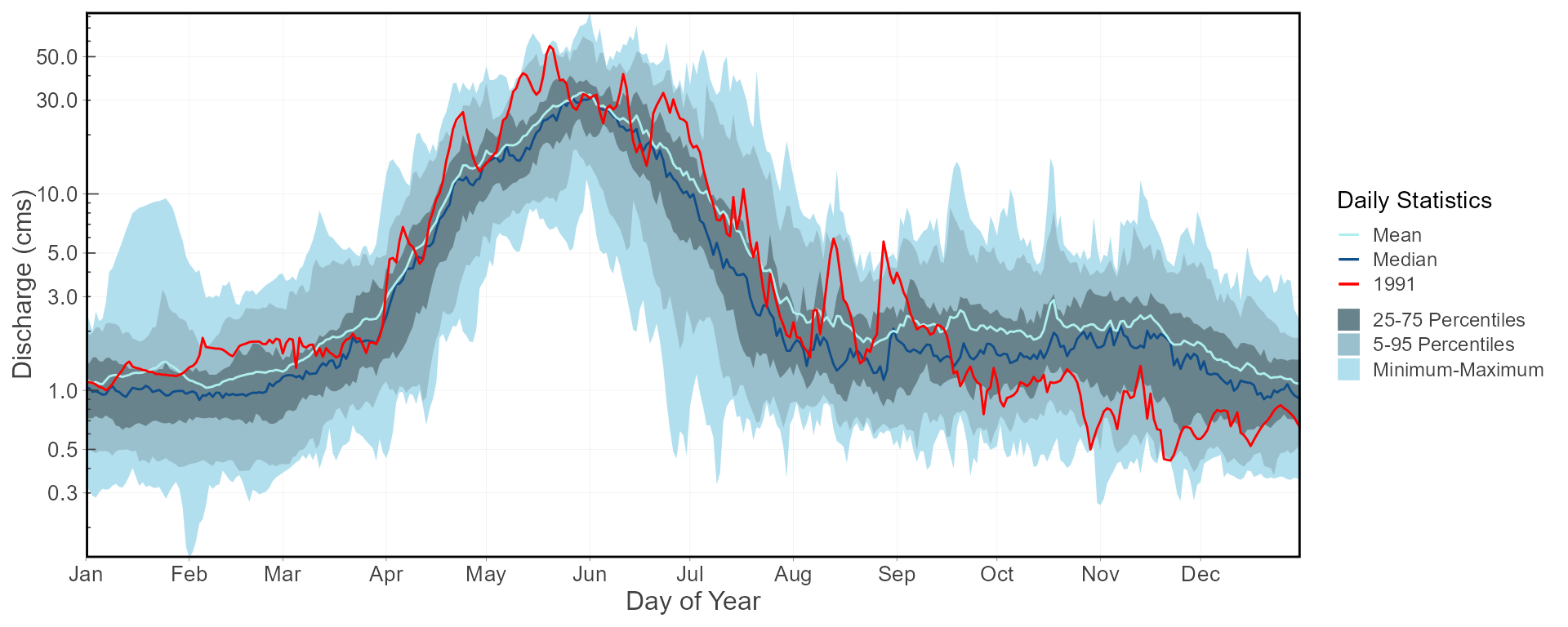
To visualize the daily streamflow patterns on an annual basis, the plot_daily_stats() function will plot out various summary statistics for each day of the year. Data can also be filtered for certain years of interest (a 1981-2010 normals period for this example) using the start_year and end_year arguments. We can also compare individual years against the statistics using add_year argument like below.

plot_daily_stats(station_number = "08NM116",
                 start_year = 1981,
                 end_year = 2010,
                 log_discharge = TRUE,
                 add_year = 1991)

## $Daily_Statistics

Plotting example: flow duration curves

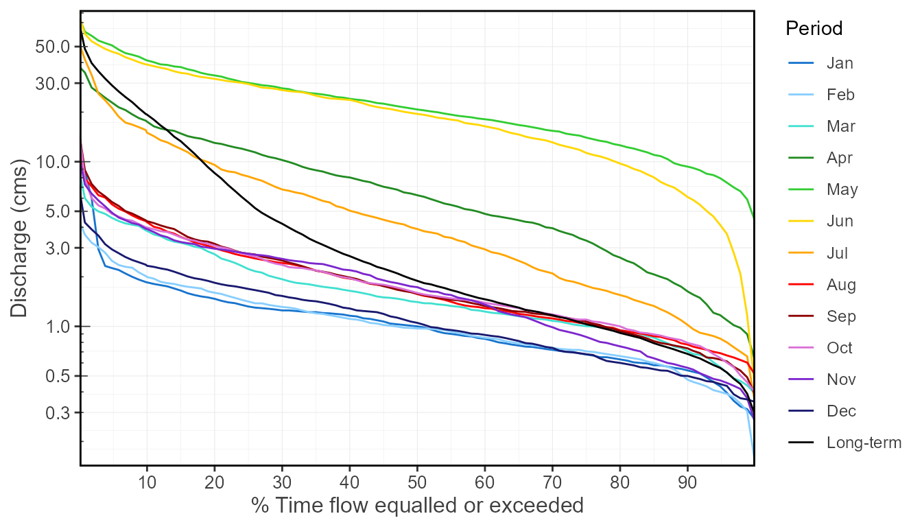
Flow duration curves can be produced using the plot_flow_duration() function.

plot_flow_duration(station_number = "08NM116",
                   start_year = 1981,
                   end_year = 2010)

## $Flow_Duration

Analysis example: low-flow frequency analysis

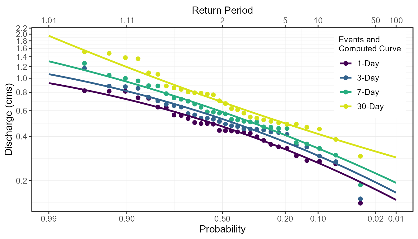
This package also provides a function, compute_annual_frequencies(), to complete a volume frequency analysis by fitting annual minimums or maximums to Log-Pearson Type III or Weibull probability distributions. See the volume frequency analyses documentation for more information. For this example, the 7-day low-flow quantiles are calculated for the Mission Creek hydrometric station using the Log-Pearson Type III distribution and method of moments fitting method (both default). With this, several low-flow indicators can be determined (i.e. 7Q5, 7Q10).

freq_results <- compute_annual_frequencies(station_number = "08NM116",
                                           start_year = 1981,
                                           end_year = 2010,
                                           roll_days = 7,
                                           fit_distr = "PIII",
                                           fit_distr_method = "MOM")
freq_results$Freq_Fitted_Quantiles

## # A tibble: 11 × 4
##    Distribution Probability `Return Period` `7-Day`
##    <chr>              <dbl>           <dbl>   <dbl>
##  1 PIII               0.01           100      0.193
##  2 PIII               0.05            20      0.277
##  3 PIII               0.1             10      0.332
##  4 PIII               0.2              5      0.408
##  5 PIII               0.5              2      0.588
##  6 PIII               0.8              1.25   0.812
##  7 PIII               0.9              1.11   0.946
##  8 PIII               0.95             1.05   1.07 
##  9 PIII               0.975            1.03   1.17 
## 10 PIII               0.98             1.02   1.21 
## 11 PIII               0.99             1.01   1.31

The probability of observed extreme events can also be plotted (using selected plotting position) along with the computed quantiles curve for comparison.

freq_results <- compute_annual_frequencies(station_number = "08NM116",
                                           start_year = 1981,
                                           end_year = 2010,
                                           roll_days = c(1,3,7,30))
freq_results$Freq_Plot