Querying Spatial Data with bcdata
2026-02-06
Source:vignettes/efficiently-query-spatial-data-in-the-bc-data-catalogue.Rmd
efficiently-query-spatial-data-in-the-bc-data-catalogue.RmdThis vignette illustrates how to use
bcdata::bcdc_query_geodata to request and query geospatial
data that has an associated Web Feature
Service from the B.C. Data Catalogue.
To illustrate, we will request and merge two spatial data sets from the
catalogue—school district and greenspaces spatial data—and then examine
the amount of park space contained within the boundaries of the Greater
Victoria, Prince George and Kamloops/Thompson British Columbia school
districts.
Getting Started
First you need to load the package. We will also load the
sf and dplyr packages to help us work with
spatial data. You can learn more about the sf package here and dplyr
here:
Geospatial Data in the B.C. Data Catalogue
The B.C. Data
Catalogue provides many data sets with spatial information through a
Web Feature
Service (WFS). Technically speaking, this means if we have an
internet connection we can issue HTTP
requests to the catalogue and seamlessly import the response data into R
as an sf objects. The bcdata package provides
a means to a) choose which layer you want and b) use dplyr
verbs to specifically tailor your request. A dbplyr backend
is implemented so that requests are executed lazily meaning results are
not transferred over the web until the user specifically calls the
collect function. This approach mimics the
dplyr verb translation to SQL seen for many
database types. A good introduction to principles of dbplyr
is available here.
School District Data
Our first step is to extract the school district polygons from the B.C. Data Catalogue. This layer is described using this command:
bcdc_get_record("78ec5279-4534-49a1-97e8-9d315936f08b")
#> B.C. Data Catalogue Record: School Districts of BC
#> Name: school-districts-of-bc (ID: 78ec5279-4534-49a1-97e8-9d315936f08b)
#> Permalink: https://catalogue.data.gov.bc.ca/dataset/78ec5279-4534-49a1-97e8-9d315936f08b
#> Licence: Open Government Licence - British Columbia
#> Description: The School Districts dataset contains the spatial representation (polygon)
#>  of the current extent of the administrative areas defined under section 176(1) of the
#>  School Act for the purposes of preservation and promotion of the fundamental principle
#>  of local autonomy and control of public education at the public and governmental levels
#>  through locally elected school boards.
#> Available Resources (1):
#>  1. WMS getCapabilities request (wms)
#> Access the full 'Resources' data frame using:
#>  bcdc_tidy_resources('78ec5279-4534-49a1-97e8-9d315936f08b')
#> Query and filter this data using:
#>  bcdc_query_geodata('78ec5279-4534-49a1-97e8-9d315936f08b')
This data is the boundary of each school district. The key
information in this metadata is that the layer has a resource in
"wms" format —which means it is available through a Web
Feature Service. From this we know we can make use of
bcdc_query_geodata.
bcdc_query_geodata("78ec5279-4534-49a1-97e8-9d315936f08b")
#> Querying 'school-districts-of-bc' record
#> • Using collect() on this object will return 59 features and 9 fields
#> • At most six rows of the record are printed here
#> ────────────────────────────────────────────────────────────────────────────────────────────────────
#> Simple feature collection with 6 features and 9 fields
#> Geometry type: POLYGON
#> Dimension:     XY
#> Bounding box:  xmin: 956376 ymin: 475108.4 xmax: 1635228 ymax: 901924.4
#> Projected CRS: NAD83 / BC Albers
#> # A tibble: 6 × 10
#>   id        ADMIN_AREA_SID SCHOOL_DISTRICT_NAME SCHOOL_DISTRICT_NUMBER FEATURE_CODE FEATURE_AREA_SQM
#>   <chr>              <int> <chr>                                 <int> <chr>                   <dbl>
#> 1 WHSE_TAN…            300 Arrow Lakes                              10 FH10000300        7392472526.
#> 2 WHSE_TAN…            301 Revelstoke                               19 FH10000300        9416076465.
#> 3 WHSE_TAN…            302 Kootenay-Columbia                        20 FH10000300        3072672101.
#> 4 WHSE_TAN…            303 Vernon                                   22 FH10000300        5588468673.
#> 5 WHSE_TAN…            304 Central Okanagan                         23 FH10000300        2916757936.
#> 6 WHSE_TAN…            305 Cariboo-Chilcotin                        27 FH10000300       61213520885.
#> # ℹ 4 more variables: FEATURE_LENGTH_M <dbl>, OBJECTID <int>, SE_ANNO_CAD_DATA <chr>,
#> #   geometry <POLYGON [m]>
This is the initial query to the data in the catalogue. What has been
returned is not the actual data but rather a subset to help you
tune your query. The printed output of this query offers several useful
pieces of information. Because we have queried with a unique ID, we are
shown the name of the record. We also receive instruction that using
collect() will retrieve a given number of features and
fields present for this query. Lastly, there is a reminder that what is
printed is only the first 6 rows of the record. Since we are limiting
the scope of analysis to the Greater Victoria, Prince George and
Kamloops/Thompson school districts, we want to ask the catalogue for
only those polygons just like we would in a typical dplyr
workflow:
bcdc_query_geodata("78ec5279-4534-49a1-97e8-9d315936f08b") %>%
  filter(SCHOOL_DISTRICT_NAME %in% c("Greater Victoria", "Prince George","Kamloops/Thompson"))
#> Querying 'school-districts-of-bc' record
#> • Using collect() on this object will return 1 features and 9 fields
#> • At most six rows of the record are printed here
#> ────────────────────────────────────────────────────────────────────────────────────────────────────
#> Simple feature collection with 1 feature and 9 fields
#> Geometry type: POLYGON
#> Dimension:     XY
#> Bounding box:  xmin: 1126789 ymin: 821142.1 xmax: 1528155 ymax: 1224202
#> Projected CRS: NAD83 / BC Albers
#> # A tibble: 1 × 10
#>   id        ADMIN_AREA_SID SCHOOL_DISTRICT_NAME SCHOOL_DISTRICT_NUMBER FEATURE_CODE FEATURE_AREA_SQM
#>   <chr>              <int> <chr>                                 <int> <chr>                   <dbl>
#> 1 WHSE_TAN…            328 Prince George                            57 FH10000300       51888780641.
#> # ℹ 4 more variables: FEATURE_LENGTH_M <dbl>, OBJECTID <int>, SE_ANNO_CAD_DATA <chr>,
#> #   geometry <POLYGON [m]>
To further tune our query, we can also request only the columns we
want. Really we only want the school district column and the spatial
information. During an actual analysis, it is possible that you may need
to initially collect more data than you want to determine value to
subset by. For example, there is currently no way to ask the catalogue
for all possible unique values of SCHOOL_DISTRICT_NAME. Is
that case the data will need to be brought into R and unique values will
need to be determined there.
bcdc_query_geodata("78ec5279-4534-49a1-97e8-9d315936f08b") %>%
  filter(SCHOOL_DISTRICT_NAME %in% c("Greater Victoria", "Prince George","Kamloops/Thompson")) %>%
  select(SCHOOL_DISTRICT_NAME)
#> Querying 'school-districts-of-bc' record
#> • Using collect() on this object will return 1 features and 5 fields
#> • At most six rows of the record are printed here
#> ────────────────────────────────────────────────────────────────────────────────────────────────────
#> Simple feature collection with 1 feature and 5 fields
#> Geometry type: POLYGON
#> Dimension:     XY
#> Bounding box:  xmin: 1126789 ymin: 821142.1 xmax: 1528155 ymax: 1224202
#> Projected CRS: NAD83 / BC Albers
#> # A tibble: 1 × 6
#>   id                             ADMIN_AREA_SID SCHOOL_DISTRICT_NAME SCHOOL_DISTRICT_NUMBER OBJECTID
#>   <chr>                                   <int> <chr>                                 <int>    <int>
#> 1 WHSE_TANTALIS.TA_SCHOOL_DISTR…            328 Prince George                            57      562
#> # ℹ 1 more variable: geometry <POLYGON [m]>
Note that in the select statement, we did not explicitly
ask for the spatial data and also that there are several columns present
that we didn’t select. This is because within each data set in the data
catalogue, there are several columns that will always be returned
regardless of what is selected. If you really don’t want those columns
after you collect the data, which we will take care of
right now, you can drop them:
districts <- bcdc_query_geodata("78ec5279-4534-49a1-97e8-9d315936f08b") %>%
  filter(SCHOOL_DISTRICT_NAME %in% c("Greater Victoria", "Prince George","Kamloops/Thompson")) %>%
  select(SCHOOL_DISTRICT_NAME) %>%
  collect()
Again note here that we have assigned the object a name and added the
collect statement. This step happens when you have selected
the data you want and wish to begin working with it in R like a normal
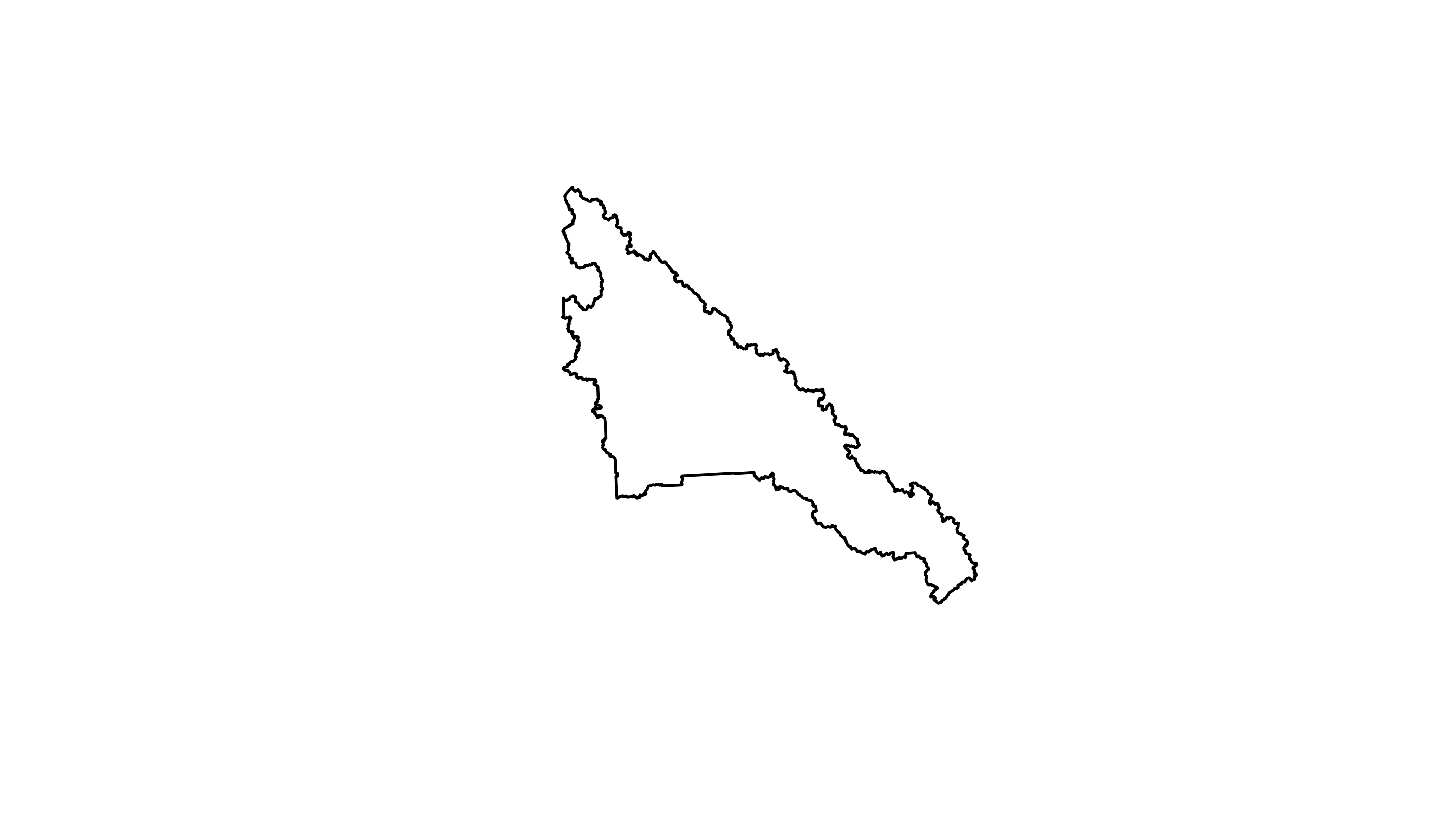
sf object. For example, we can now plot these three school
districts:
plot(st_geometry(districts))
plot of chunk districts
Now that we have the spatial boundaries narrowed by specific school districts we can perform some spatial operations to determine parks in the school districts.
Greenspaces Data
For the purposes of this example, let’s consider this greenspace layer in the catalogue. This layer is described here:
bcdc_get_record("6a2fea1b-0cc4-4fc2-8017-eaf755d516da")
#> B.C. Data Catalogue Record: Local and Regional Greenspaces
#> Name: local-and-regional-greenspaces (ID: 6a2fea1b-0cc4-4fc2-8017-eaf755d516da)
#> Permalink: https://catalogue.data.gov.bc.ca/dataset/6a2fea1b-0cc4-4fc2-8017-eaf755d516da
#> Licence: Open Government Licence - British Columbia
#> Description: This dataset contains spatial and attribute information for local and
#>  regional greenspaces in British Columbia. Local and regional greenspaces are municipal
#>  or regional district lands designated by local government agencies and managed for
#>  public enjoyment, ecosystem or wildlife values. Spatial boundaries were sourced from
#>  municipal and regional district web sites, which in some cases provide datasets under
#>  Open Government Licence, and in other cases, publicize parks and greenspaces on web maps
#>  or pdf maps. Boundaries were edge-matched to the ParcelMap BC cadastre.  This spatial
#>  layer contains multipart polygons.
#> Available Resources (2):
#>  1. WMS getCapabilities request (wms)
#>  2. LocalRegionalParksAttributeValues (xlsx)
#> Access the full 'Resources' data frame using:
#>  bcdc_tidy_resources('6a2fea1b-0cc4-4fc2-8017-eaf755d516da')
#> Query and filter this data using:
#>  bcdc_query_geodata('6a2fea1b-0cc4-4fc2-8017-eaf755d516da')
Again we recognize this is WFS-enabled
geospatial data, which means we can make use of
bcdc_query_geodata.
bcdc_query_geodata("6a2fea1b-0cc4-4fc2-8017-eaf755d516da")
#> Querying 'local-and-regional-greenspaces' record
#> • Using collect() on this object will return 9212 features and 19 fields
#> • At most six rows of the record are printed here
#> ────────────────────────────────────────────────────────────────────────────────────────────────────
#> Simple feature collection with 6 features and 19 fields
#> Geometry type: POLYGON
#> Dimension: XY
#> Bounding box: xmin: 1205933 ymin: 459093.3 xmax: 1212220 ymax: 460485.6
#> Projected CRS: NAD83 / BC Albers
#> # A tibble: 6 × 20
#> id LOCAL_REG_GREENSPACE…¹ PARK_NAME PARK_TYPE PARK_PRIMARY_USE REGIONAL_DISTRICT MUNICIPALITY
#> <chr> <int> <chr> <chr> <chr> <chr> <chr>
#> 1 WHSE_B… 49 Woodward… Local Park Metro Vancouver Richmond
#> 2 WHSE_B… 50 Woodward… Local Park Metro Vancouver Richmond
#> 3 WHSE_B… 51 Doggie P… Local Park Metro Vancouver Richmond
#> 4 WHSE_B… 52 Bike Ter… Local Athletic Metro Vancouver Richmond
#> 5 WHSE_B… 53 Great We… Local Trail Metro Vancouver Richmond
#> 6 WHSE_B… 54 Imperial… Local Park Metro Vancouver Richmond
#> # ℹ abbreviated name: ¹LOCAL_REG_GREENSPACE_ID
#> # ℹ 13 more variables: CIVIC_NUMBER <int>, CIVIC_NUMBER_SUFFIX <chr>, STREET_NAME <chr>,
#> # LATITUDE <dbl>, LONGITUDE <dbl>, WHEN_UPDATED <date>, WEBSITE_URL <chr>,
#> # LICENCE_COMMENTS <chr>, FEATURE_AREA_SQM <dbl>, FEATURE_LENGTH_M <dbl>, OBJECTID <int>,
#> # SE_ANNO_CAD_DATA <chr>, geometry <POLYGON [m]>Since we are interested in only “Park” data we can subset our query:
bcdc_query_geodata("6a2fea1b-0cc4-4fc2-8017-eaf755d516da") %>%
filter(PARK_PRIMARY_USE == "Park")
#> Querying 'local-and-regional-greenspaces' record
#> • Using collect() on this object will return 4528 features and 19 fields
#> • At most six rows of the record are printed here
#> ────────────────────────────────────────────────────────────────────────────────────────────────────
#> Simple feature collection with 6 features and 19 fields
#> Geometry type: POLYGON
#> Dimension: XY
#> Bounding box: xmin: 1205029 ymin: 459093.3 xmax: 1212220 ymax: 461188.7
#> Projected CRS: NAD83 / BC Albers
#> # A tibble: 6 × 20
#> id LOCAL_REG_GREENSPACE…¹ PARK_NAME PARK_TYPE PARK_PRIMARY_USE REGIONAL_DISTRICT MUNICIPALITY
#> <chr> <int> <chr> <chr> <chr> <chr> <chr>
#> 1 WHSE_B… 49 Woodward… Local Park Metro Vancouver Richmond
#> 2 WHSE_B… 50 Woodward… Local Park Metro Vancouver Richmond
#> 3 WHSE_B… 51 Doggie P… Local Park Metro Vancouver Richmond
#> 4 WHSE_B… 54 Imperial… Local Park Metro Vancouver Richmond
#> 5 WHSE_B… 55 Stevesto… Local Park Metro Vancouver Richmond
#> 6 WHSE_B… 56 Mariner'… Local Park Metro Vancouver Richmond
#> # ℹ abbreviated name: ¹LOCAL_REG_GREENSPACE_ID
#> # ℹ 13 more variables: CIVIC_NUMBER <int>, CIVIC_NUMBER_SUFFIX <chr>, STREET_NAME <chr>,
#> # LATITUDE <dbl>, LONGITUDE <dbl>, WHEN_UPDATED <date>, WEBSITE_URL <chr>,
#> # LICENCE_COMMENTS <chr>, FEATURE_AREA_SQM <dbl>, FEATURE_LENGTH_M <dbl>, OBJECTID <int>,
#> # SE_ANNO_CAD_DATA <chr>, geometry <POLYGON [m]>Here we see that this greatly reduces the number of features that we
are dealing with (and correspondingly the amount of data that needs to
be transferred over the web). Remember also that we still have not
actually requested the full data set. This is just still a preview. Also
this query still includes all municipal parks in BC while we only want
the ones in the three school districts - the polygons defined by the
districts object. To find that subset of parks we can make
use of the built-in geometric operators which allow us to perform
spatial operations remotely fine tuning our query even further. Here
using the INTERSECTS function is appropriate and since this
is a last tuning step, we can call collect and assign a
name to this object. These requests can sometimes take quite a long:
districts_parks <- bcdc_query_geodata("6a2fea1b-0cc4-4fc2-8017-eaf755d516da") %>%
  filter(PARK_PRIMARY_USE == "Park") %>%
  filter(INTERSECTS(districts)) %>%
  collect()
#> The object is too large to perform exact spatial operations using bcdata.
#> Object size: 948576 bytes
#> BC Data Threshold: 500000 bytes
#> Exceedance: 448576 bytes
#> See ?bcdc_check_geom_size for more details
#> A bounding box was drawn around the object passed to INTERSECTS and all features within the box will be returned.
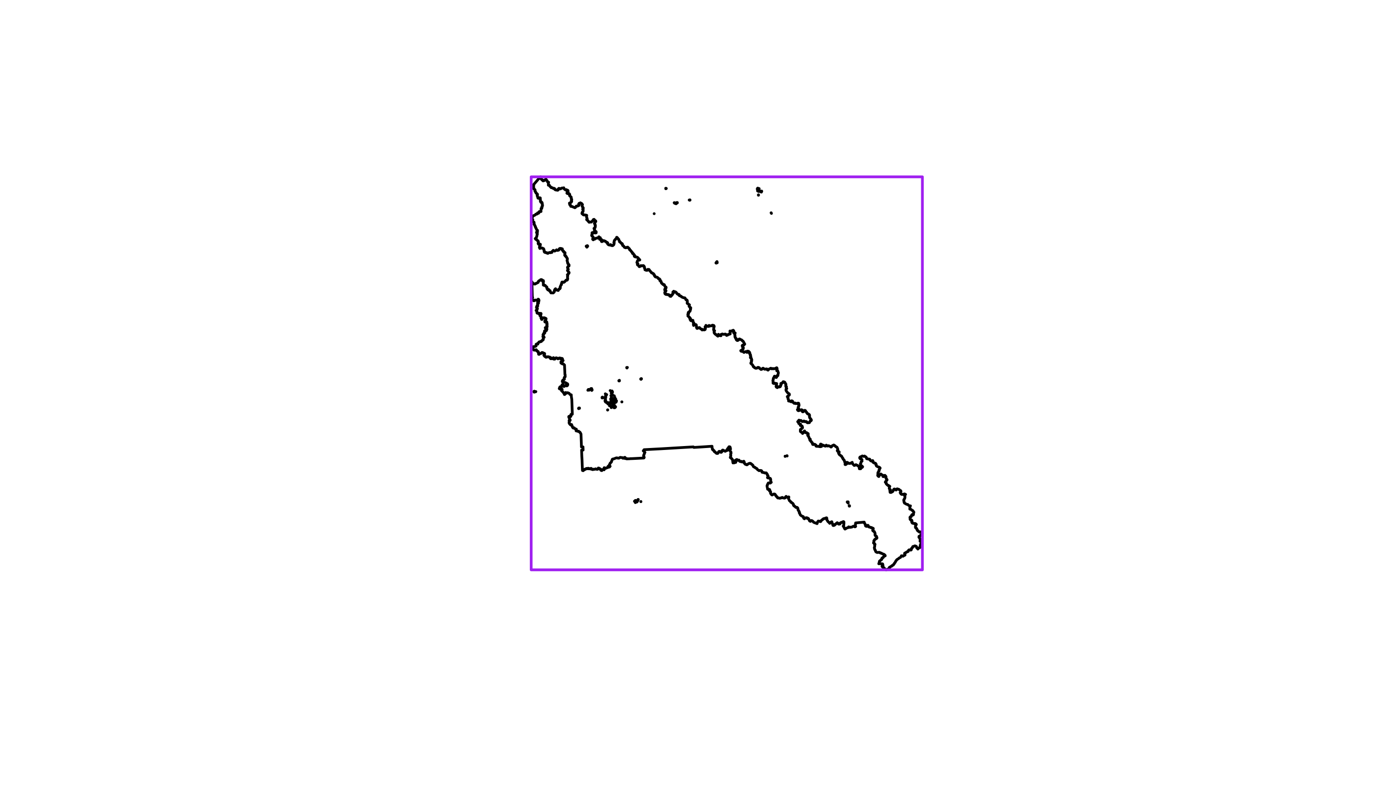
Plotting both the filtered parks data and the district polygons
reveals an important consideration when using bcdata:

plot of chunk district_parks
In this example, many parks not contained within the school districts
are included in the districts_parks object. This is because
rather than a full intersection, bcdata draws a bounding
box around all the polygons that are doing the intersection (in this
case district) and does the intersection based on that
bounding box. This behaviour is imposed by the Web Feature Server but
controlled via the bcdata.max_geom_pred_size option (See
?bcdc_options for default values). Using this example, you
can check to see if the size of the districts object
exceeded the current value of
bcdata.max_geom_pred_size:
bcdc_check_geom_size(districts)
#> The object is too large to perform exact spatial operations using bcdata.
#> Object size: 948576 bytes
#> BC Data Threshold: 500000 bytes
#> Exceedance: 448576 bytes
#> See ?bcdc_check_geom_size for more details
Drawing the bounding box illustrates this point:

plot of chunk bbox
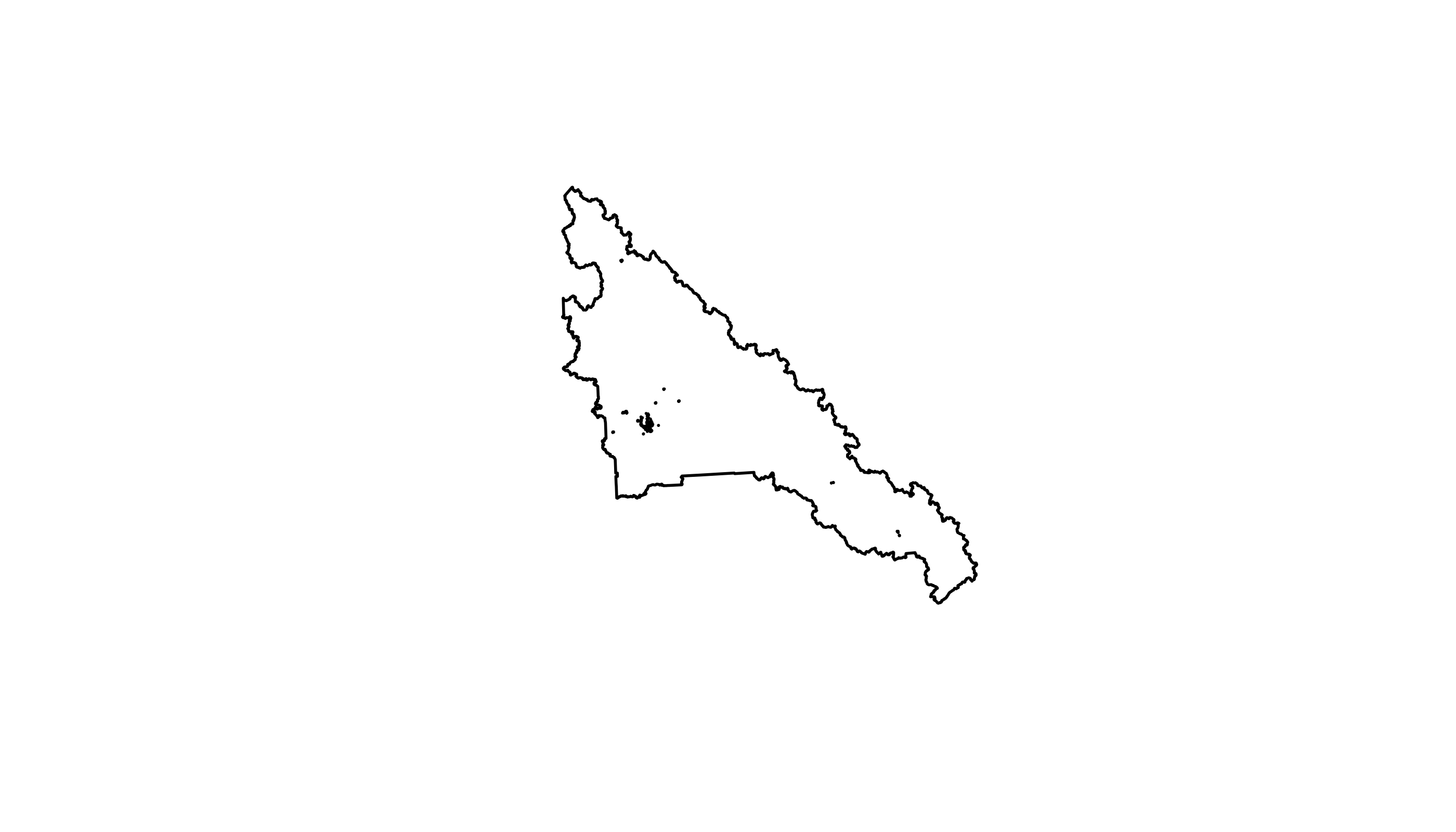
We are left with two options to get around this problem. First, we
can simply do some additional processing with the sf
package. Specifically we can use a spatial join to assign parks into
their respective district:

plot of chunk dp_join
A second approach is to set an internal option
(bcdata.max_geom_pred_size) and increase the threshold of
when a bounding box is drawn. Options are set in R like this:
The value of bcdata.max_geom_pred_size is set
conservatively so that requests to the Web Feature Service are more
consistently successful. Increasing this value may result in invalid
requests.
Finally, to address our original question of which school district has the most municipal park space we can calculate the area of each park polygon and then sum those areas by school district:
districts_parks_join %>%
  mutate(area = st_area(geometry)) %>%
  st_set_geometry(NULL) %>%
  group_by(SCHOOL_DISTRICT_NAME) %>%
  summarise(total_area = sum(area)) %>%
  arrange(total_area)
#> # A tibble: 1 × 2
#>   SCHOOL_DISTRICT_NAME total_area
#>   <chr>                     [m^2]
#> 1 Prince George         11793481.
A note about using local R functions in constructing filter queries
Suppose we now want to find all of the parks within 1km of the school
districts we are interested in. We can use sf::st_buffer()
to make a buffer around the districts object, then
intersect that with the greenspaces data. Note that
st_buffer() needs to be executed in R on our computer, to
create the buffered area that is sent to the WFS server to perform the
INTERSECT query remotely. We tell filter() to
evaluate that piece of code locally by wrapping it in a
local() call:
greenspaces_around <- bcdc_query_geodata("6a2fea1b-0cc4-4fc2-8017-eaf755d516da") %>%
  filter(INTERSECTS(local(st_buffer(districts, 1000)))) %>%
  collect()
Additional Useful Functions
There are a couple of other functions in bcdata that are
useful to know when working with spatial data from the catalogue.
bcdc_describe_feature gives the column names, whether the
column is selectable, and the column types in both R and on the remote
server:
bcdc_describe_feature("6a2fea1b-0cc4-4fc2-8017-eaf755d516da")
#> # A tibble: 20 × 5
#>    col_name                sticky remote_col_type          local_col_type column_comments
#>    <chr>                   <lgl>  <chr>                    <chr>          <chr>
#>  1 id                      TRUE   xsd:string               character      <NA>
#>  2 LOCAL_REG_GREENSPACE_ID TRUE   xsd:decimal              numeric        LOCAL_REG_GREENSPACE_ID i…
#>  3 PARK_NAME               FALSE  xsd:string               character      PARK NAME is the name of …
#>  4 PARK_TYPE               FALSE  xsd:string               character      PARK_TYPE is the type of …
#>  5 PARK_PRIMARY_USE        FALSE  xsd:string               character      PARK PRIMARY USE defines …
#>  6 REGIONAL_DISTRICT       FALSE  xsd:string               character      REGIONAL_DISTRICT is the …
#>  7 MUNICIPALITY            FALSE  xsd:string               character      MUNICIPALITY is the name …
#>  8 CIVIC_NUMBER            FALSE  xsd:decimal              numeric        CIVIC_NUMBER is the stree…
#>  9 CIVIC_NUMBER_SUFFIX     FALSE  xsd:string               character      CIVIC_NUMBER_SUFFIX is th…
#> 10 STREET_NAME             FALSE  xsd:string               character      STREET_NAME is the name o…
#> 11 LATITUDE                FALSE  xsd:decimal              numeric        LATITUDE is the geographi…
#> 12 LONGITUDE               FALSE  xsd:decimal              numeric        LONGITUDE is the geograph…
#> 13 WHEN_UPDATED            FALSE  xsd:date                 date           WHEN_UPDATED is the date …
#> 14 WEBSITE_URL             FALSE  xsd:string               character      WEBSITE_URL contains a li…
#> 15 LICENCE_COMMENTS        FALSE  xsd:string               character      LICENCE_COMMENTS describe…
#> 16 FEATURE_AREA_SQM        FALSE  xsd:decimal              numeric        FEATURE_AREA_SQM is the s…
#> 17 FEATURE_LENGTH_M        FALSE  xsd:decimal              numeric        FEATURE_LENGTH_M is the s…
#> 18 SHAPE                   FALSE  gml:GeometryPropertyType sfc geometry   SHAPE is the column used …
#> 19 OBJECTID                TRUE   xsd:decimal              numeric        OBJECTID is a column requ…
#> 20 SE_ANNO_CAD_DATA        FALSE  xsd:hexBinary            numeric        SE_ANNO_CAD_DATA is a bin…
This is a helpful initial step to learn column names and types when you construct your query.
Another useful function is show_query() which provides
information on the request issued to the remote server:
bcdc_query_geodata("6a2fea1b-0cc4-4fc2-8017-eaf755d516da") %>%
  filter(PARK_PRIMARY_USE == "Park") %>%
  filter(INTERSECTS(districts)) %>%
  show_query()
#> <url>
#> <body>
#> SERVICE: WFS VERSION: 2.0.0 REQUEST: GetFeature outputFormat: application/json typeNames:
#>  WHSE_BASEMAPPING.GBA_LOCAL_REG_GREENSPACES_SP SRSNAME: EPSG:3005 CQL_FILTER:
#>  (("PARK_PRIMARY_USE" = 'Park') AND (INTERSECTS(SHAPE, POLYGON ((1126789 821142.1,
#>  1528155 821142.1, 1528155 1224202, 1126789 1224202, 1126789 821142.1)))))
#>
#> <full query url>
#> https://openmaps.gov.bc.ca/geo/pub/wfs?SERVICE=WFS&VERSION=2.0.0&REQUEST=GetFeature&outputFormat=application%2Fjson&typeNames=WHSE_BASEMAPPING.GBA_LOCAL_REG_GREENSPACES_SP&SRSNAME=EPSG%3A3005&CQL_FILTER=%28%28%22PARK_PRIMARY_USE%22%20%3D%20%27Park%27%29%20AND%20%28INTERSECTS%28SHAPE%2C%20POLYGON%20%28%281126789%20821142.1%2C%201528155%20821142.1%2C%201528155%201224202%2C%201126789%201224202%2C%201126789%20821142.1%29%29%29%29%29
This output is what being created by the dplyr code outlined above.
Using B.C. Geographic Warehouse (BCGW) layer names
If you are familiar with the B.C.
Geographic Warehouse (BCGW), you may already know the name of a
layer that you want from the BCGW. bcdc_query_geodata() (as
well as all other related functions) supports supplying that name
directly. For example, the record
for the B.C. airports layer shows that the object name is
WHSE_IMAGERY_AND_BASE_MAPS.GSR_AIRPORTS_SVW, and we can use
that in bcdc_query_geodata():
# Look at the columns available:
bcdc_describe_feature("WHSE_IMAGERY_AND_BASE_MAPS.GSR_AIRPORTS_SVW")
#> # A tibble: 42 × 5
#> col_name sticky remote_col_type local_col_type column_comments
#> <chr> <lgl> <chr> <chr> <chr>
#> 1 id TRUE xsd:string character <NA>
#> 2 CUSTODIAN_ORG_DESCRIPTION TRUE xsd:string character CUSTODIAN_ORG_DESCRIPTION co…
#> 3 BUSINESS_CATEGORY_CLASS TRUE xsd:string character BUSINESS_CATEGORY_CLASS desi…
#> 4 BUSINESS_CATEGORY_DESCRIPTION TRUE xsd:string character BUSINESS_CATEGORY_DESCRIPTIO…
#> 5 OCCUPANT_TYPE_DESCRIPTION TRUE xsd:string character OCCUPANT_TYPE_DESCRIPTION co…
#> 6 SOURCE_DATA_ID TRUE xsd:string character SOURCE_DATA_ID is a unique o…
#> 7 SUPPLIED_SOURCE_ID_IND TRUE xsd:string character SUPPLIED_SOURCE_ID_IND is an…
#> 8 AIRPORT_NAME TRUE xsd:string character AIRPORT_NAME is a business n…
#> 9 DESCRIPTION FALSE xsd:string character DESCRIPTION describes the Oc…
#> 10 PHYSICAL_ADDRESS FALSE xsd:string character PHYSICAL_ADDRESS contains th…
#> # ℹ 32 more rows
# Query the data with bcdc_query_geodata and filter + select:
bcdc_query_geodata("WHSE_IMAGERY_AND_BASE_MAPS.GSR_AIRPORTS_SVW") %>%
filter(DESCRIPTION == "airport") %>%
select(AIRPORT_NAME, LOCALITY, NUMBER_OF_RUNWAYS)
#> Querying 'WHSE_IMAGERY_AND_BASE_MAPS.GSR_AIRPORTS_SVW' record
#> • Using collect() on this object will return 37 features and 11 fields
#> • At most six rows of the record are printed here
#> ────────────────────────────────────────────────────────────────────────────────────────────────────
#> Simple feature collection with 6 features and 11 fields
#> Geometry type: POINT
#> Dimension: XY
#> Bounding box: xmin: 833428.6 ymin: 406147 xmax: 1264896 ymax: 1055403
#> Projected CRS: NAD83 / BC Albers
#> # A tibble: 6 × 12
#> id CUSTODIAN_ORG_DESCRI…¹ BUSINESS_CATEGORY_CL…² BUSINESS_CATEGORY_DE…³ OCCUPANT_TYPE_DESCRI…⁴
#> <chr> <chr> <chr> <chr> <chr>
#> 1 WHSE_… "Ministry of Forest, … airTransportation Air Transportation BC Airports
#> 2 WHSE_… "Ministry of Forest, … airTransportation Air Transportation BC Airports
#> 3 WHSE_… "Ministry of Forest, … airTransportation Air Transportation BC Airports
#> 4 WHSE_… "Ministry of Forest, … airTransportation Air Transportation BC Airports
#> 5 WHSE_… "Ministry of Forest, … airTransportation Air Transportation BC Airports
#> 6 WHSE_… "Ministry of Forest, … airTransportation Air Transportation BC Airports
#> # ℹ abbreviated names: ¹CUSTODIAN_ORG_DESCRIPTION, ²BUSINESS_CATEGORY_CLASS,
#> # ³BUSINESS_CATEGORY_DESCRIPTION, ⁴OCCUPANT_TYPE_DESCRIPTION
#> # ℹ 7 more variables: SOURCE_DATA_ID <chr>, SUPPLIED_SOURCE_ID_IND <chr>, AIRPORT_NAME <chr>,
#> # LOCALITY <chr>, NUMBER_OF_RUNWAYS <int>, SEQUENCE_ID <int>, geometry <POINT [m]>