ShinyRems Users Guide

ShinyRems is an online application that allows a user to view, clean, plot and calculate simple statistics using water quality data from the B.C. government Environmental Monitoring System (EMS) database.

Using the App

• The shinyrems app is in a completed phase, however like any application bugs do occur. If the app greys out and/or freezes, reload the internet browser. If that doesn’t fix the issue, close the web browser, revisit RStudio and rerun the launch code to restart the app.

• The app requires Chrome or Firefox internet browsers to run. If Internet Explorer is the users default internet browser, once the app opens in Internet Explorer, the user can copy and paste the web link into Chrome or Firefox.

• Once the app opens in the users’ web browser, go through the tabs sequentially as each tab depends on the previous for information. The user can go back a tab to make changes if necessary, without restarting at tab 1.

• In the app: variable = parameter, limit = guideline

• A key feature of the app, and to keep track of the changes that occur to the dataset each tab, a data download option is available after each stage of data manipulation from raw, tidying, cleaning, outlier removal, plotting and summary statistics.

• Blue question mark circles are present throughout the app to explain what each option is asking and how those choices will affect the dataset.

Getting Started

This app must be launched from the RStudio program. The app then opens in the users’ computer’s internet browser. Given the EMS database is so large, the app accesses EMS data cached on the users’ computer and why the app cannot be directly opened from a web link.

Download R and R Studio

The latest versions of the computer programs R and RStudio are essential to running the app. See this website for how to install the latest versions of R and RStudio on a BC government workstation.

Launch ShinyRems App

Once R and RStudio are installed on the users’ computer, there are two options for getting the R code to launch the app:

1. View the README at this website to follow the instructions to launch the app. Copy and paste the code into a new R Script file within RStudio: File -> New File -> R Script (Figure 1).

2. Contact Heather Thompson (heather.c.thompson@gov.bc.ca) or Karly Harker (karly.harker@gov.bc.ca) for existing R scripts containing the code in Figure 1 to launch the app.

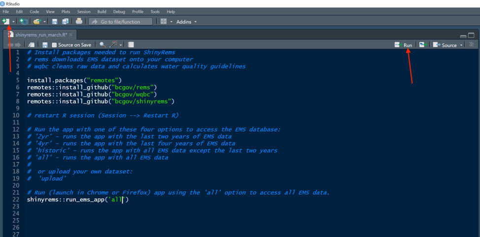Figure 1: R code script in the RStudio program. This is the code to run to open the shinyrems app.

When initially launching the app, it is recommended to run each line of code by itself. Line 6 in Figure 1 will cache the latest versions of the EMS database onto the users’ computer. This will take awhile. Further help is at this website if needed.

There are six options for running the app, depending what year of EMS data is required:

• demo’ - uses a demo dataset that requires no download of EMS data

• ‘2yr’ - uses the most recent 2 years of EMS data

• ‘4yr’ - uses the most recent 4 years of EMS data

• ‘historic’ - uses the historic EMS data (1965 - (Current Year - 2 Years))

• ‘all’ - uses combined “2yr” and “historic” EMS data

• ‘upload’ - allows user to upload their own data following correct format. For details see “Using the upload data option” section below.

See the BC Data Catalogue for more information about the EMS datasets.

Pick the option required and type it into line 22 as shown in Figure 1 or below. Press the ‘Run’ button on the RStudio menu bar (Figure 1). The app will open in the users’ web browser. For example, the line of code below will launch the app with all EMS data.

shinyrems::run_ems_app('all')

After running line 22 above, Figure 2 and Figure 3 show the questions asked in the RStudio console and require the users input. When the text “Listening on http…”, this means the app has launched in the users’ internet browser.

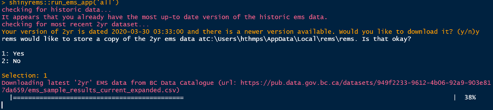Figure 2. A message to answer when the code to launch the app is run. The ‘2yr’ EMS dataset is updated every day.

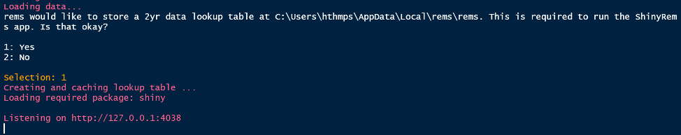Figure 3. A message to answer when the code to launch the app is run. This message confirms a data look up table can be stored on the users’ computer.

ShinyRems App Features

Tab 1: Data

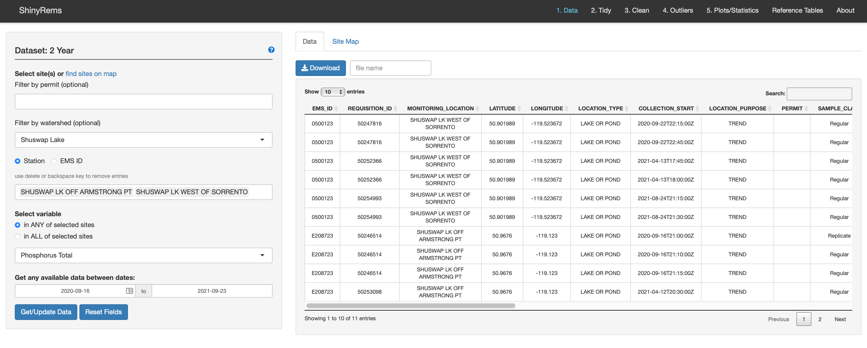Figure 4. The first screen seen when the app opens in the users web browser. The dataset chosen in the R code will be listed in the top left. Raw data can be chosen multiple ways, with options to view one parameter at a time and at a specific date range.

Using 2yr, 4yr, historic or all options

When the app opens, Figure 4 is the initial app screen. The dataset chosen in the R code will be displayed in the top left of the screen. In the left-hand menu, the options for choosing the raw EMS dataset are:

1. By permit number.

2. By monitoring location or EMS ID. Multiple entries can be entered.

3. The Site Map inset tab (Figure 3) can be used to find a monitoring location. Clicking a marker will add the site to the users list of selected sites. An option to zoom to Freshwater Atlas watershed groups is available.

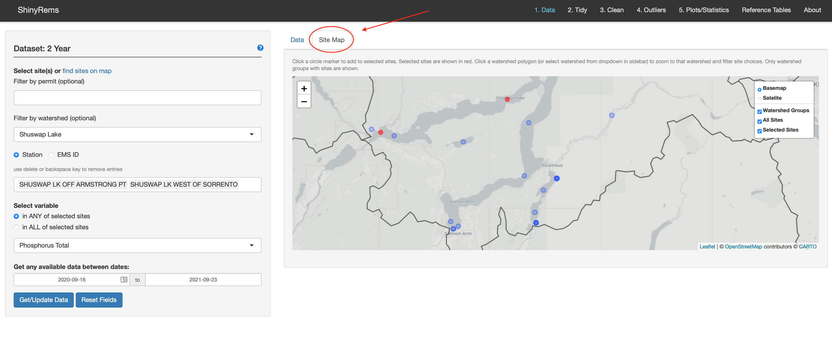Figure 5. Raw data can also be found by selecting monitoring site locations on the Site Map inset tab.

One parameter can be chosen at a time for the site(s) selected. In ANY of selected sites means that the parameters could be in one or more of the sites, in ALL of selected sites, the parameter list updates to what parameters are found in all the sites.

A date range can be specified. Note this has bounds depending on the ‘2yr’, ‘4yr’ and/or ‘historic’ dataset chosen.

The Get/Update Data button will need to be pushed if changes are made to the data input choices.

The raw data from EMS appears in the inset Data tab. Raw data is shown with a subset of 21 columns pertaining to water quality data:

EMS_ID, MONITORING_LOCATION, LATITUDE, LONGITUDE, LOCATION_TYPE, COLLECTION_START, LOCATION PURPOSE, PERMIT, SAMPLE_CLASS, SAMPLE_STATE, SAMPLE_DESCRIPTOR, PARAMETER_CODE, PARAMETER, ANALYTICAL_METHOD_CODE, ANALYTICAL_METHOD, RESULT_LETTER, RESULT, UNIT, METHOD_DETECTION_LIMIT, MDL_UNIT, QA_INDEX_CODE, UPPER_DEPTH, LOWER_DEPTH.  

A download raw data button exists to keep track of the raw dataset. Make sure to name it something descriptive.

Using the upload data option

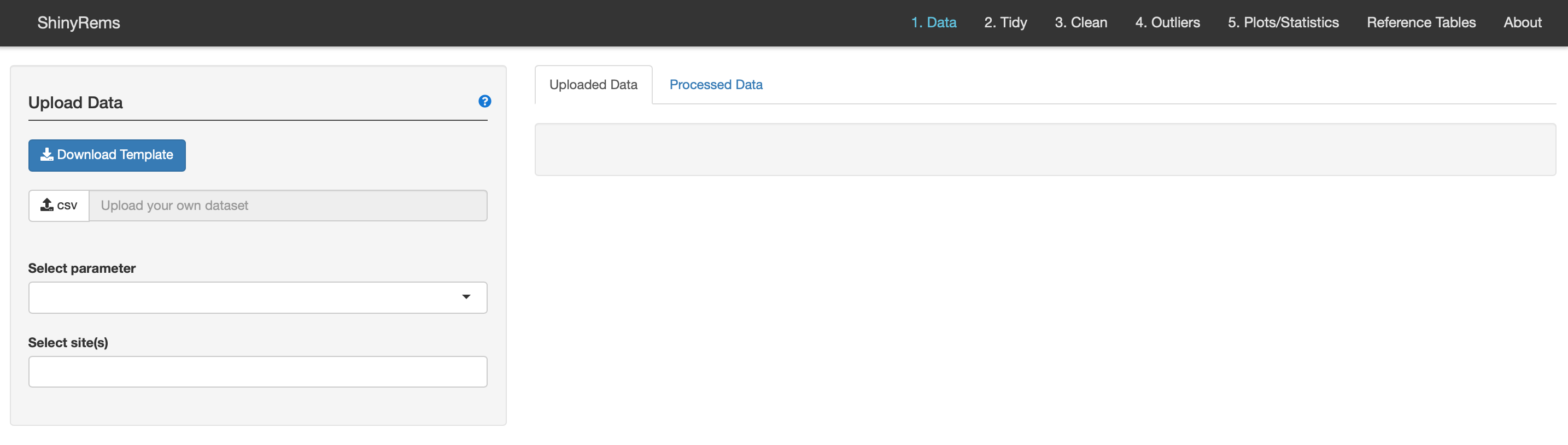Figure 6. The first screen the user will see when the app opens in the users web browser when the ‘upload’ option is chosen.

If the user wants to upload a dataset not from EMS, choose the option ‘upload’:

shinyrems::run_ems_app('upload')

When the app opens, instructions pop up outlining the format the dataset must be in to upload to shinyrems:

Instructions

Uploading a dataset

Download a template for data entry with the ‘Download Template’ button in the sidebar. When your data is uploaded, the app will check that column names are valid and that constraints are met (e.g. Month must be a number between 1 and 12). Any columns in addition to those that are mandatory will simply be accepted and passed through the app.

The following columns are mandatory:

• Station
  • Name of the station
• Year
  • Year of measurement
• Month
  • Month of measurement as number from 1 - 12
• Day
  • Day of measurement as number from 1 - 31
• Variable
  • Variable of measurement (e.g. parameter name)
• Value
  • Value of measurement as number
• Units
  • Unit of measurement

The following columns are optional and can be used by the app:

• DetectionLimit
  • Detection limit as number
• ResultLetter
  • Result letter, e.g. (<)
• EMS_ID
  • EMS ID corresponding to Station
• Hour
  • Hour of measurement in 24-hour clock as number from 0 - 23
• Minute
  • Minute of measurement as number from 0 - 59
• Second
  • Second of measurement as number from 0 - 59

Figure 6 is the screen the user will see when the ‘upload’ version of shinyrems opens. The user can download the template to view what format the data needs to be in (Figure 7).

Data must be in a .csv file to upload into the app. Excel workbooks formats are not accepted. If the datafile is an excel file, export a worksheet to csv.

Figure 7. Template of how the users’ data needs to be organized to upload into app.

Tab 2. Tidy

This step does two main things:

• Retains and renames required columns (e.g. PARAMETER to Variable) (Figure 8).
  • Columns are simplified to 15. The default columns retained are:
    • “EMS_ID”
    • “MONITORING_LOCATION” (Renamed to “Station”)
    • “COLLECTION_START” (Renamed to “DateTime”)
    • “PARAMETER” (Renamed to “Variable”)
    • “PARAMETER_CODE” (Renamed to “Code”)
    • “RESULT” (Renamed to “Value”)
    • “UNIT” (Renamed to “Units”)
    • “METHOD_DETECTION_LIMIT” (Renamed to “DetectionLimit”)
    • “RESULT_LETTER” (Renamed to “ResultLetter”)
    • “SAMPLE_STATE”
    • “SAMPLE_CLASS”
    • “SAMPLE_DESCRIPTOR”
• Sets the timezone to PST
• Filter out unwanted values of SAMPLE_CLASS and SAMPLE_STATE (e.g. blanks and replicates)

The Tidy Tab manual options for tidying the dataset include (Figure 9):

1. Select which SAMPLE_STATE to include in dataset. The options present in the dataset will automatically show up. For more information see the Reference Tables Tab. Options include:
   • Fresh Water
     
   • Waste Water
     
   • HiVol
     
   • HiVol Selective Size Inlet
     
   • Air Emission
     
   • Dustfall
     
   • Stack
     
   • Soil
     
   • Animal Tissue
     
   • Ground Water
     
   • Refuse
     
   • Marine Water
     
   • Plant Tissue
2. Select which SAMPLE_CLASS to include in dataset. The options present in the dataset will automatically show up. See the Reference Tables Tab for more information. Options include:
   • Blank
   • Regular
     
   • Replicate
     
   • Replicate - Sequential
   • Replicate-First
     
   • Replicate-Second
     
   • Replicate - Paired
3. Set values at or below detection limit gives an option what to do with data points below the detection limit. Options are converting result value to zero, half the detection limit, setting at the minimum detection limit or to set as NA.

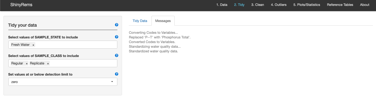Figure 8. The Messages inset tab of the Tidy Tab. This shows what is happening automatically in the Tidy Tab.

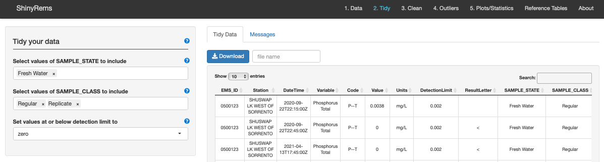Figure 9. Tab 2 in ShinyRems. This tab is where the users raw data starts to be tidied and includes a few automatic and manual steps to customize the users dataset.

Tab 3. Clean

This step does the following:

• Checks that all variables in the Variable column can be recognized (see Parameters table in Reference Tables tab), and if necessary, replaces the variable name with a recognized one.
• Removes negative values and standardizes units. Units are changed to what the aquatic life water quality guideline is reported in.
• Calculates a summary value (max, mean or median) for replicates, which are defined as two or more readings for the same variable on the same date. Data can also be summarized by additional columns such as Station.
• Replaces DateTime column with Date (YYYY-MM-DD)

The Clean Tab options for cleaning the dataset include (Figure 10):

1. Summarize by columns retains columns in the dataset. For example, if the user is assessing lake data, retaining UPPER_DEPTH and LOWER_DEPTH columns will likely be important to view data collected on the same day but at different depths. If the user simply wants to plot and summarize data by EMS_ID, just retain the EMS_ID column.

2. Summarize by function gives an option of how the replicates can be summarized. Replicates are counted as two or more samples for the same variable on the same day. If the user has retained SAMPLE_CLASS = Replicate, these will be included with SAMPLE_CLASS = Regular in summarizing the same day samples. Options to summarize by ‘mean’, ‘median’, and ‘max’.

3. Maximum Coefficient of Variation for replicates is an option to specify the coefficient of variation between sample replicates. Replicates are counted as two or more samples for the same variable on the same day. Leave blank for the default value of infinity.

Figure 10. The main screen of the Clean Tab. This is where various options exist for cleaning the users now tidy dataset.

Tab 4. Outliers

This step calculates potential outliers. Outliers can also be manually removed by clicking on the plot. Colour indicates outliers, Symbol indicates if observation is <MDL (i.e., True).

1. Standard deviations is an option to specify the number of standard deviations above which a data point is considered an outlier.

2. Ignore values below detection limit is an option to specify whether to ignore data points below the detection limit when calculating the average deviation and calculating outliers.

3. Large values only is an option to select whether only values which exceed the specified number of expected standard deviations should be identified as outliers. For example, any values less than the mean by the selected number of standard deviations will not be considered outliers.

4. Remove outliers from plot. Choose whether to view the plot with or without outliers. Regardless, the outliers are removed from the dataset before moving onto the next tab.

5. Plot customizations: Point size and plot height.

6. Manual outlier removal: Click and drag mouse over a data point on the plot to manually select and remove outliers. This will remove it from the dataset.

7. Number of columns: Choose number of columns to ‘facet’ plots side by side. 1 column will put plots of top of each other, 2 will place plots side by side.

8. Plot legend: Outliers are identified by colour. Data are identified as Detected – True (above minimum detection limit) or Detected - False (below minimum detection limit; with a < in the Result Letter column).

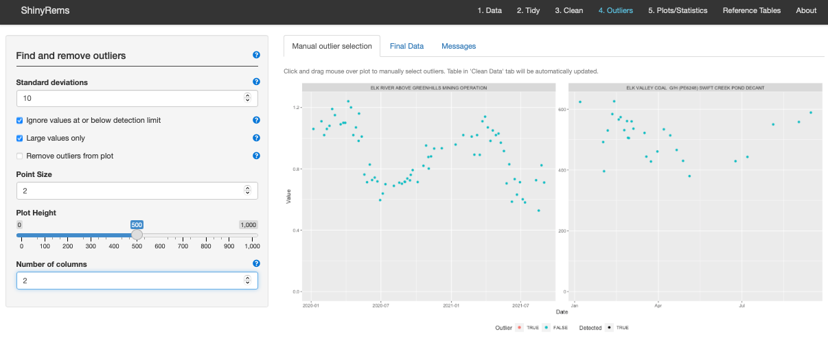Figure 11. The main tab of the Outlier screen. Options here include customizing what constitutes an outlier for the dataset and removing them if desired.

Final clean data with outliers removed can be downloaded as a .csv (Figure 12).

Figure 12. The main screen of the Outliers Tab showing the Final Data inset tab. This shows the final clean dataset with outliers removed.

Tab 5. Plots/Statistics

The Plots/Statistics tab allows for the initial visualization of the clean dataset with the addition of the aquatic life water quality guideline if desired, and a simple statistics summary.

Plot Tab

Figure 13 shows the main Plot tab, with options for customization:

1. Adjusting plot start and end date.
   
2. Plot type: scatter or boxplot with options to show lines and/or points.
   
3. Point size and line size.
   
4. Facet by Variable to have the various EMS_IDs show up on the same plot, or Facet by EMS_ID to show one plot each for each EMS_ID.
   
5. Colour by allows for options to colour by variable or EMS_ID.
   
6. Plot height allows the plot to get larger.
   
7. Palette allows for colour customization.
8. Number of columns allows for setting number of columns for faceting plots.
9. Standardize Y-axis scales allows user to specify whether you would like the y-axis scales to be standardized (i.e. “fixed”) or not (i.e. “free”).

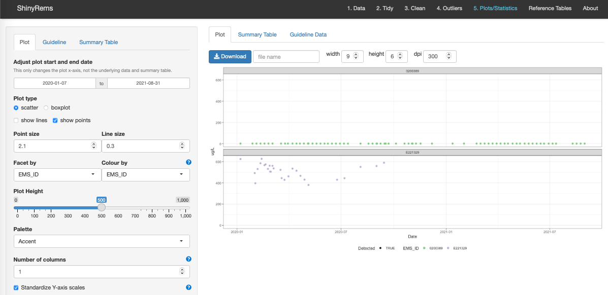Figure 13. The main plot screen. Here the user can view the initial visualization of the clean dataset with outliers removed. Various options exist for customizing the plot and downloading it to the users computer.

Guideline Tab

There are two options:

Set manually

Any benchmark value may be entered here. Examples include permit limits, water quality objectives, or water quality guidelines that are not calculated. See Limits in the Reference Tables tab or visit the Water Quality Guideline look-up table.

Calculate from data

Calculates the approved water quality guidelines for aquatic life in British Columbia (Figure 14). Only guidelines whose conditions are met are returned.

The aquatic life guidelines and their details can be found under the ‘Limits’ drop-down menu on the Reference Tables tab. All BC approved water quality guidelines are also available on the BC ambient water quality guidelines website and DataBC. Two options may be set by the user: ‘Term’ and ‘Get modelled estimate’.

Term:

Term options include ‘short’, ‘long’ and ‘long-daily’.

For long-term limits there must be at least 5 values spanning 21 days. As replicates are averaged prior to calculating the limits each of the 5 values must be on a separate day. The first 30-day period begin at the date of the first reading while the next 30 day period starts at the date of the first reading after the previous period and so on. The only exception to this is if the user provides dates in which case each period extends for 30 days or until a provided date is reached. It is important to note that the averaging of conditional variables, the 5 in 30 rule and the assignment of 30-day periods occurs independently for all combination of factor levels in the columns specified by.

‘Long-daily’ term uses long-term guidelines on daily values; 5 samples in 30 days is not required to calculate guideline.

Get modelled estimate:

A limit may depend on another variable such as pH, Total Chloride, or Total Hardness and in some cases no value was recorded for the date of interest.

If the ‘Get modelled estimate box’ is unchecked:

The pH, Total Chloride or Total Hardness value is assumed to be the average recorded value over the 30 day period.

If the ‘Get modelled estimate box’ is checked:

A parametric model is used to predict the pH, Total Chloride and Total Hardness for all dates with a value of any variable. Existing values are replaced. If, in every year, there are less then 12 pH/Total Chloride/Total Hardness then an average value is taken. Otherwise, if there is only one year with 12 or more values a simple seasonal smoother is used. If there is two years with 12 or more values then a seasonal smoother with a trend is fitted. Otherwise, a model with trend and a dynamic seasonal component is fitted.

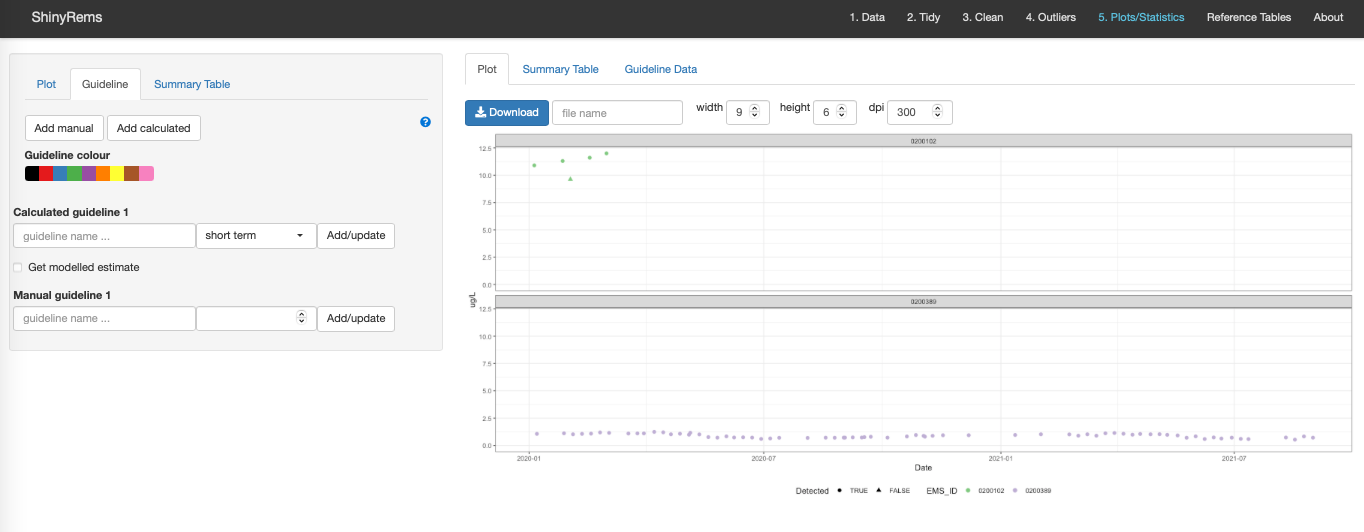Figure 14. The Guideline inset tab showing the options for calculating the aquatic life guideline of the variable selected in the 1. Data tab.

Summary Table Tab

The Summary Table options allow for calculation of a summary table which can be downloaded as a .csv. The Summary Table gives a simple stats summary for each EMS_ID based on the clean dataset with outliers removed (Figure 15). Columns include n (number of water samples), ncen (number of censored values), min (minimum water value), max (maximum water value), mean (mean water value), median (median water value), lowerQ (25%), upperQ (75%), sd, se, lower CL and upper CL.

Accounting for censored data (data at or below the detection limit) involves treating the value at face value when calculating the summary table or accounting for these non-detects using left-censored log-normal maximum-likelihood.

An option to exclude missing values in the ‘Value’ column when summarizing data. Options also exist to decide which column to summarize the data by and how many significant figures are wanted.

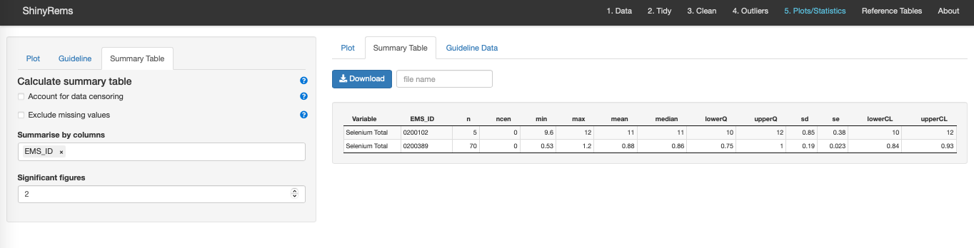Figure 15. The summary table tab in the main Tab 5. Plot/Statistics.

Tab 6: Reference Tables

Tab 6 shows the various EMS reference tables. These include information for each EMS column and its respective options. These tables will be helpful in Tab 2, 3 and 5 as the dataset is refined and guidelines are calculated.

Figure 16. The Reference Tables tab which show all options for the various EMS columns. These show the EMS reference tables available from Data BC.

Resources

• Water quality guidelines

• Water quality objectives (can be entered into the app in the ‘set manually’ option)

• Analyzing water quality data resources

• EMS training and manual (intranet)

• Surface water monitoring sites map

• Water data and tools webpage