Chapter 9 Dataframe Manipulation with tidyr
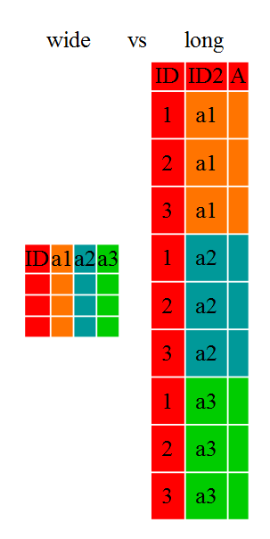
Researchers often want to manipulate their data from the ‘wide’ to the ‘long’ format, or vice-versa. The ‘long’ format is where:
- each column is a variable
- each row is an observation
In the ‘long’ format, you usually have 1 column for the observed variable and the other columns are ID variables.
For the ‘wide’ format each row is often a site/subject/patient and you have
multiple observation variables containing the same type of data. These can be
either repeated observations over time, or observation of multiple variables (or
a mix of both). You may find data input may be simpler or some other
applications may prefer the ‘wide’ format. However, many of R‘s functions have
been designed assuming you have ’long’ format data. This tutorial will help you
efficiently transform your data regardless of original format.
These data formats mainly affect readability. For humans, the wide format is often more intuitive since we can often see more of the data on the screen due to its shape. However, the long format is more machine readable and is closer to the formatting of databases. The ID variables in our dataframes are similar to the fields in a database and observed variables are like the database values.
9.1 Getting started
First install the packages if you haven’t already done so (you probably installed dplyr in the previous lesson):
Load the packages
First, lets look at the structure of our original gapminder dataframe:
Parsed with column specification:
cols(
  country = col_character(),
  year = col_double(),
  pop = col_double(),
  continent = col_character(),
  lifeExp = col_double(),
  gdpPercap = col_double()
)# A tibble: 1,704 x 6
country year pop continent lifeExp gdpPercap
<chr> <dbl> <dbl> <chr> <dbl> <dbl>
1 Afghanistan 1952 8425333 Asia 28.8 779.
2 Afghanistan 1957 9240934 Asia 30.3 821.
3 Afghanistan 1962 10267083 Asia 32.0 853.
4 Afghanistan 1967 11537966 Asia 34.0 836.
5 Afghanistan 1972 13079460 Asia 36.1 740.
6 Afghanistan 1977 14880372 Asia 38.4 786.
7 Afghanistan 1982 12881816 Asia 39.9 978.
8 Afghanistan 1987 13867957 Asia 40.8 852.
9 Afghanistan 1992 16317921 Asia 41.7 649.
10 Afghanistan 1997 22227415 Asia 41.8 635.
# … with 1,694 more rows9.1 Challenge 1
Is gapminder a purely long, purely wide, or some intermediate format?
9.1 Solution to Challenge 1
The original gapminder data.frame is in an intermediate format. It is not purely long since it had multiple observation variables (
pop,lifeExp,gdpPercap).
Sometimes, as with the gapminder dataset, we have multiple types of observed
data. It is somewhere in between the purely ‘long’ and ‘wide’ data formats. We
have 3 “ID variables” (continent, country, year) and 3 “Observation
variables” (pop,lifeExp,gdpPercap). This intermediate format can be
preferred despite not having ALL observations in 1 column given that all 3
observation variables have different units. There are few operations that would
need us to stretch out this dataframe any longer (i.e. 4 ID variables and 1
Observation variable).
While using many of the functions in R, which are often vector based, you
usually do not want to do mathematical operations on values with different
units. For example, using the purely long format, a single mean for all of the
values of population, life expectancy, and GDP would not be meaningful since it
would return the mean of values with 3 incompatible units. The solution is that
we first manipulate the data either by grouping (see the lesson on dplyr), or
we change the structure of the dataframe. Note: Some plotting functions in
R actually work better in the wide format data.
9.2 Convert long format with gather()
Here we have used piping syntax which is similar to what we were doing in the previous lesson with dplyr. In fact, these are compatible and you can use a mix of tidyr and dplyr functions by piping them together
Inside gather() we first name the new column for the new ID variable and then
the value column taking the country, year and continent variables out
of the gathering process:
Inside spread() we have the opposite situation where we take the vars column and spread
it over to separate columns with value filling those cells:
9.3 Advantage to plotting and tables
Reshaping your data from wide to long provides considerable flexibility for
presenting your results. Combining some dplyr grouping code with tidyr
we can produce a nice table:
gapminder %>%
    gather(key = vars, value = value, -country, -year, -continent) %>%
    group_by(continent, vars) %>%
    summarise(total_pop = sum(value)) %>%
    spread(key = continent, value = total_pop)
# A tibble: 3 x 6
vars Africa Americas Asia Europe Oceania
<chr> <dbl> <dbl> <dbl> <dbl> <dbl>
1 gdpPercap 1368903. 2140833. 3129252. 5209011. 446919.
2 lifeExp 30492. 19398. 23786. 25885. 1784.
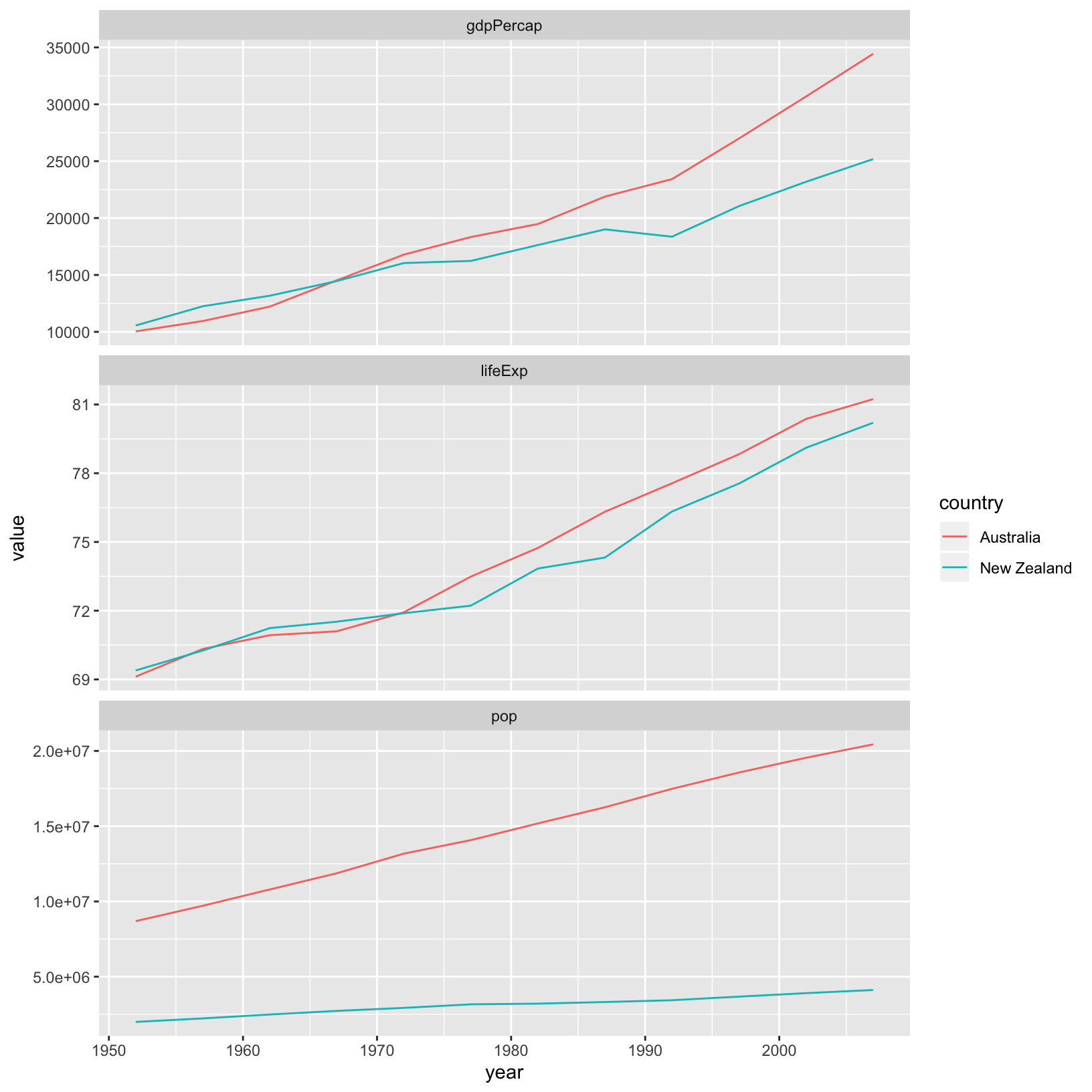
3 pop 6187585961 7351438499 30507333902. 6181115304 212992136 Similarly, gathering can provide considerable more flexibility when plotting by grouping variables we might want to facet as well as using some additional dplyr content:
library(ggplot2)

gapminder_long %>%
    filter(continent == "Oceania") %>%
    ggplot(aes(x = year, y = value, colour = country)) +
    geom_line() +
    facet_wrap(~vars, scales = "free_y", ncol = 1)