PEMprepr

library(PEMprepr)
library(ggplot2)
library(sf)
library(terra)

PEMprepr, short for Predictive Ecosystem Mapping – Preparation is the first of a series of packages supporting the British Columbia Biogeoecosystem Classification’s
Predictive Ecosystem Mapping (PEM) project. See BC-BEC and PEMr on _GitHub_for details about the BC BEC classification system and, the PEM Project.

A portion of the Aleza Lake Research Forest, one of the pilot study sites for this project, is used for this example. The area outlined in red will be used in the steps below

In the example below it is assumed that you are running the following within a new R project.

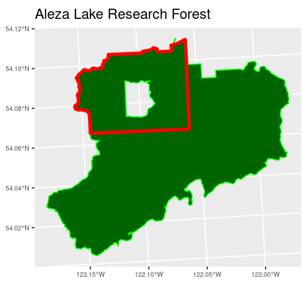
The Aleza Lake Research forest with the area of interest outlined in red

Workflow

The following provides a standard workflow for preparing data for subsequent sampling, modeling, and mapping. The key steps demonstrated below include:

Data folder set up.
Alignment of the area of interest
Generation of covariates
Creation of a multi-resolution raster stack
Collection of vector data.

Folder setup

Data for the project can quickly become difficult to manage. To facilitate ease of data management a standard set of folders for each area of interest. The following creates the needed folders for the area of interest: aleza. In addition, fstr stores a named list of the folders created which we will utilize later (e.g. to programmatically place results of functions in the correct place).

_Note: if the folders have been generated previously this function will still return the list of folder names.

# creates dirs and returns a named list
fstr <- setup_folders("aleza",            
                      full_names = FALSE) # relative or full path

str(fstr[1:5]) ## first 5 in the list. 
#> [1] "The aleza folder already exists - returning folder names."
#> List of 5
#>  $ AOI_dir      : chr "aleza"
#>  $ raw_dir      : chr "aleza/00_raw_inputs"
#>  $ shape_raw_dir: chr "aleza/00_raw_inputs/vector/raw"
#>  $ derived_dir  : chr "aleza/10_map_inputs"
#>  $ cov_dir      : chr "aleza/10_clean_inputs/covariates"

Alignment of the area of interest

Load the spatial data

aoi   <- sf::st_read(system.file("extdata/aleza_nw.gpkg", 
                                 package = "PEMprepr"), quiet = TRUE)

sf::st_bbox(aoi) ## note extent
#>    xmin    ymin    xmax    ymax 
#> 1250797 1013823 1257215 1019097

One concern, with this area-of-interest (aoi) (red area) is that the bounding box or geographic extent of the area ends with very random numbers (output above). Using this extent will cause significant problems later when we attempt to stack numerous rasters.

Snap the extent

Here the aoi is snapped to an extent divisible by 100. This will facilitate the generation of rasters data that all fits this grid extent and thereby can be stacked with relative ease.

aoi <- aoi_snap(aoi, method = "shrink") ## or expand
#> [1] "initial extent is:"
#>    xmin    ymin    xmax    ymax 
#> 1250797 1013823 1257215 1019097 
#> [1] "Extent is:"
#>    xmin    ymin    xmax    ymax 
#> 1250800 1013900 1257200 1019000

Raster templates

The snapped aoi can now be used to create a raster template. In the example below a 25m² raster template is created.

t25 <- create_template(aoi, 25)
t25 ## note that the extent of the raster is the same as the aoi. 
#> class       : SpatRaster 
#> dimensions  : 204, 256, 1  (nrow, ncol, nlyr)
#> resolution  : 25, 25  (x, y)
#> extent      : 1250800, 1257200, 1013900, 1019000  (xmin, xmax, ymin, ymax)
#> coord. ref. : NAD83 / BC Albers (EPSG:3005) 
#> source      : memory 
#> name        : lyr.1 
#> min value   :     0 
#> max value   :     0

Generation of covariates

Here we generate the terrain derived covariates. This is powered by SAGA-GIS. Covariates are generated at multiple resolutions, for example 5, 10, and 25m².

Steps to create the covariates

load a digital terrain model (dtm). Generally, this will be a high resolution model derived from lidar.
align the dtm to the template. resample the dtm to the desired resolution – here we demonstrate using the 25m² templated created above.
create the covariates

Import the terrain model

dtm <- terra::rast(system.file("extdata/aleza_nw.tif",
                               package = "PEMprepr"))
dtm
#> class       : SpatRaster 
#> dimensions  : 1170, 1408, 1  (nrow, ncol, nlyr)
#> resolution  : 5.000284, 5.000422  (x, y)
#> extent      : 1250480, 1257520, 1013524, 1019375  (xmin, xmax, ymin, ymax)
#> coord. ref. : NAD83 / BC Albers (EPSG:3005) 
#> source      : aleza_nw.tif 
#> name        : aleza_nw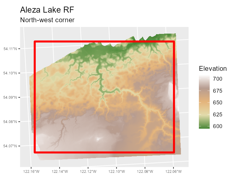

A raw digital terrain model with the area-of-interest noted in red. All processed rasters will align with the aoi.

Align the raster

dtm25 <- align_raster(dtm, t25)
dtm25
#> class       : SpatRaster 
#> dimensions  : 204, 256, 1  (nrow, ncol, nlyr)
#> resolution  : 25, 25  (x, y)
#> extent      : 1250800, 1257200, 1013900, 1019000  (xmin, xmax, ymin, ymax)
#> coord. ref. : NAD83 / BC Albers (EPSG:3005) 
#> source      : memory 
#> name        : aleza_nw 
#> min value   : 595.0263 
#> max value   : 704.1022

Create the covariates

layer_options <- 
  c("Filled_sinks", "sinkroute", "dem_preproc", 
    "slope_aspect_curve", "tCatchment", "tca", "sCatchment", 
    "twi", "channelsNetwork", "Distance2Water", 
    "MultiResFlatness", "MultiResFlatness2",
    "MultiResFlatness3", "TRI", "convergence", "Openness",
    "dah", "TPI", "RidgeValley", "MRN", "FlowAccumulation",
    "SlopeLength", "FlowAccumulation2", "FlowAccumulation3",
    "FlowPathLength", "FlowPathLength2", "FlowPathLength3", 
    "LSFactor", "SolarRad", "Convexity", "VertDistance", "TCI_low",
    "SWI", "WindExp", "Texture", "Protection", "VRM",
    "MBI", "mscale_TPI", "RelPosition", "SlopeCurvatures",
    "SteepestSlope", "UpslopeArea")



create_covariates(dtm = dtm25,           ## raster created above
                  SAGApath = "c:/SAGA/", ## Where SAGA GIS is installed
                  output = fstr$cov_dir, ## from the setup_folders above
                  layers = "all")        ## use all or one of the above

Note that the pre-defined output directory fstr$cov_dir, created using setup_folders(), is used to ensure generated covariates are saved to the correct location. Rasters are also saved into subfolders of the same resolution.

l <- list.files(path = fstr$cov_dir, pattern = ".sdat",
                recursive = TRUE)
l <- l[!grepl("xml",l)]

## created covariates 
head(l, 20)

#>  [1] "25/aspect.sdat"              
#>  [2] "25/cnetwork.sdat"            
#>  [3] "25/convergence.sdat"         
#>  [4] "25/convexity.sdat"           
#>  [5] "25/dah.sdat"                 
#>  [6] "25/dem_preproc.sdat"         
#>  [7] "25/diffinso.sdat"            
#>  [8] "25/direinso.sdat"            
#>  [9] "25/down_curv.sdat"           
#> [10] "25/dtm.sdat"                 
#> [11] "25/Filled_sinks.sdat"        
#> [12] "25/flow_accum_ft.sdat"       
#> [13] "25/flow_accum_p.sdat"        
#> [14] "25/flow_accum_td.sdat"       
#> [15] "25/flowlength1.sdat"         
#> [16] "25/FlowPathLenTD.sdat"       
#> [17] "25/gencurve.sdat"            
#> [18] "25/hdistnob.sdat"            
#> [19] "25/local_curv.sdat"          
#> [20] "25/local_downslope_curv.sdat"

Note: As SAGA-GIS is used the files resulting files are all saved in .sdat format – this is read/writable by terra::rast

Creation of the multi-resolution raster stack

Generation of the covariates above is repeated for each resolution in the multi-resolution model. In order to make all of the rasters stackable, necessary for model and map generation, they must all have the same extent and resolution.

The process above ensures they all have the same extent.

Next the coarse resolution rasters are disaggregated to a fine scale resolution. This means that the data in the resulting raster is the data of the coarse-raster but in a fine scale format.

Note: it is highly recommended to use full.names = TRUE to list the files.

## we can use the list of files from above
l <- list.files(path = fstr$cov_dir,
                pattern = ".sdat",
                full.names = TRUE, ## Use TRUE
                recursive = TRUE)
l <- l[!grepl("xml",l)]


create_fine_res(inputFileList = l[1:5],     ## using the list of files above  
                output = fstr$cov_dir, ## from setup_folders())
                targetRes = 5)

#> [1] "Processing: aleza/10_clean_inputs/covariates/25/aspect.sdat"
#> [1] "Created: aleza/10_clean_inputs/covariates/5/aspect_25.sdat"
#> [1] "Processing: aleza/10_clean_inputs/covariates/25/cnetwork.sdat"
#> [1] "Created: aleza/10_clean_inputs/covariates/5/cnetwork_25.sdat"
#> [1] "Processing: aleza/10_clean_inputs/covariates/25/convergence.sdat"
#> [1] "Created: aleza/10_clean_inputs/covariates/5/convergence_25.sdat"
#> ...

This script is a wrapper for terra::disaggregate.

Collection of vector data

A standard set of Vector data is used for subsequent sample planning and is based on the aoi. This script collects numerous vector layers from the BC Data Catalogue making use of the bcdata package

create_base_vectors(in_aoi = aoi,
                    out_path = fstr$shape_raw_dir)

files are saved in geopackage format.

Example workflow