Easily generate scatterplots using ggplot2 with a simplified customization interface for common modifications with static (ggplot) and interactive (plotly) output options. The static output is useful for producing static reports (e.g. for manuscripts) and is readily customized further using ggplot2 syntax. The interactive output is helpful for exploring the data and producing dynamic html reports. See this blog post for an introduction to ggplot2.
plot_scatter(
  data,
  y,
  x,
  jitter = FALSE,
  shape = 21,
  ...,
  fill_var = NULL,
  colour_var = NULL,
  shape_var = NULL,
  size_var = NULL,
  ylab = NULL,
  xlab = NULL,
  title = NULL,
  title_hjust = 0.5,
  caption = NULL,
  caption_hjust = 0,
  fill_var_title = NULL,
  colour_var_title = NULL,
  shape_var_title = NULL,
  size_var_title = NULL,
  ylim = c(NA, NA),
  ybreaks = ggplot2::waiver(),
  transform_y = FALSE,
  y_transformation = "log10",
  y_var_labs = ggplot2::waiver(),
  xlim = c(NA, NA),
  xbreaks = ggplot2::waiver(),
  transform_x = FALSE,
  x_transformation = "log10",
  x_var_labs = ggplot2::waiver(),
  size_lim = c(NA, NA),
  transform_size = FALSE,
  size_transformation = "log10",
  fill_var_order = NULL,
  colour_var_order = NULL,
  shape_var_order = NULL,
  fill_var_labs = NULL,
  colour_var_labs = NULL,
  shape_var_labs = NULL,
  fill_var_values = NULL,
  colour_var_values = NULL,
  shape_var_values = NULL,
  palette = c("plasma", "C", "magma", "A", "inferno", "B", "viridis", "D", "cividis",
    "E"),
  palette_direction = c("d2l", "l2d"),
  palette_begin = 0,
  palette_end = 0.8,
  regression_line = FALSE,
  regression_method = "gam",
  regression_formula = NULL,
  regression_se = FALSE,
  ci_level = 0.95,
  regression_geom = "smooth",
  regression_line_size = 1,
  regression_line_colour = NULL,
  regression_alpha = 0.5,
  regression_line_type = 1,
  regression_line_full_range = FALSE,
  regression_method_args = NULL,
  loess_span = 0.75,
  alpha = 0.6,
  greyscale = FALSE,
  theme = c("bw", "classic", "grey", "light", "dark", "minimal"),
  text_size = 14,
  font = c("sans", "serif", "mono"),
  facet_var = NULL,
  facet_var_order = NULL,
  facet_var_labs = NULL,
  facet_var_strip_position = c("top", "bottom"),
  facet_var_text_bold = TRUE,
  legend_position = c("right", "left", "top", "bottom"),
  omit_legend = FALSE,
  interactive = FALSE,
  aesthetic_options = FALSE
)
Arguments
- data
A data frame or tibble containing the dependent measure "y", the independent measure "x", and any grouping variables or covariates.
- y
A numeric variable you want to plot against x (quoted or unquoted), e.g. y = "variable" or y = variable.
- x
A numeric variable you want to plot against y (quoted or unquoted), e.g. x = "variable" or x = variable.
- jitter
Set to TRUE to slightly offset overlapping points in random directions. See
geom_jitterfor details.- shape
Point shape to use. Default is 21 for "circle filled". Use the "aesthetic_options" argument to view the options.
- ...
graphical parameters (not associated with variables) to be passed to
geom_point, e.g. colour or fill, to be applied to all bars. To see some of the available options in a web browser, set the aesthetic_options argument to TRUE.- fill_var
Use if you want to assign a variable to the point fill colour, e.g. fill_var = "grouping_variable" or fill_var = grouping_variable. Produces separate sets of points for each level of the fill variable. See
aesfor details. Note: for geom_point, fill_var and fill only affect shapes 21-24. To split the data by a variable based on colour, it is therefore easier to use colour_var for this particular plot geometry. Also works with continuous variables.- colour_var
Use if you want to assign a variable to the point outline colour, e.g. colour_var = "grouping_variable" or colour_var = grouping_variable. Produces separate sets of points for each level of the colour variable. See
aesfor details.- shape_var
Use if you want to assign a variable to the point shape, e.g. shape_var = "grouping_variable" or shape_var = grouping_variable. Produces separate sets of points for each level of the shape variable. See
aesfor details.- size_var
Use if you want to assign a continuous variable to the point size, e.g. size_var = "covariate" or size_var = covariate. Adjusts point sizes according to the value of the covariate. See
aesfor details.- ylab
Specify/overwrite the y-axis label using a character string, e.g. "y-axis label"
- xlab
Specify/overwrite the x-axis label using a character string, e.g. "x-axis label"
- title
Add a main title to the plot using a character string, e.g. "scatterplot of y as a function of x"
- title_hjust
Left-to-right/horizontal justification (alignment) of the main plot title. Accepts values from 0 (far left) to 1 (far right). Default is 0.5 (centre).
- caption
Add a figure caption to the bottom of the plot using a character string.
- caption_hjust
Left-to-right/horizontal justification (alignment) of the caption. Accepts values from 0 (far left) to 1 (far right). Default is 0 (left).
- fill_var_title
If a variable has been assigned to fill using fill_var, this allows you to modify the variable label in the plot legend.
- colour_var_title
If a variable has been assigned to colour using colour_var, this allows you to modify the variable label in the plot legend.
- shape_var_title
If a variable has been assigned to shape using shape_var, this allows you to modify the variable label in the plot legend.
- size_var_title
If a variable has been assigned to shape using shape_var, this allows you to modify the variable label in the plot legend.
- ylim
specify the y-axis limits, e.g. ylim = c(lower_limit, upper_limit). Use NA for the existing minimum or maximum value of y, e.g. the default is ylim = c(NA, NA).
- ybreaks
This allows you to change the break points to use for tick marks on the y-axis.
seqis particularly useful here. Seescale_y_continuousfor details. If ybreaks is specified, then ylim should be also.- transform_y
Would you like to transform the y axis? (TRUE or FALSE)
- y_transformation
If transform_y = TRUE, this determines the transformation to be applied. Common choices include "log10" (the default), "log2", "sqrt", or "exp". See
scale_continuousfor details.- y_var_labs
Allows you to modify the labels displayed with the y-axis tick marks. See
scale_continuousfor details.- xlim
specify the x-axis limits, e.g. xlim = c(lower_limit, upper_limit). Use NA for the existing minimum or maximum value of x, e.g. the default is xlim = c(NA, NA)
- xbreaks
This allows you to change the break points to use for tick marks on the x-axis.
seqis particularly useful here. Seescale_x_continuousfor details. If xbreaks is specified, then xlim should be also.- transform_x
Would you like to transform the x axis? (TRUE or FALSE)
- x_transformation
If transform_x = TRUE, this determines the transformation to be applied. Common choices include "log10" (the default), "log2", "sqrt", or "exp". See
scale_continuousfor details.- x_var_labs
Allows you to modify the labels displayed with the x-axis tick marks. See
scale_continuousfor details.- size_lim
specify the size scale limits, e.g. size_lim = c(lower_limit, upper_limit). Use NA for the existing minimum or maximum value of x, e.g. the default is size_lim = c(NA, NA)
- transform_size
Would you like to transform the size scale? (TRUE or FALSE)
- size_transformation
If transform_size = TRUE, this determines the transformation to be applied. Common choices include "log10" (the default), "log2", "sqrt", or "exp". See
scale_continuousfor details.- fill_var_order
If a variable has been assigned to fill using fill_var, this allows you to modify the order of the variable groups, e.g. fill_var = grouping_variable, fill_var_order = c("group_2", "group_1"). See
fct_relevelfor details.- colour_var_order
If a variable has been assigned to colour using colour_var, this allows you to modify the order of the variable groups, e.g. colour_var = grouping_variable, fill_var_order = c("group_2", "group_1"). See
fct_relevelfor details.- shape_var_order
If a variable has been assigned to shape using shape_var, this allows you to modify the order of the variable groups, e.g. shape_var = grouping_variable, shape_var_order = c("group_2", "group_1"). See
fct_relevelfor details.- fill_var_labs
If a variable has been assigned to fill using fill_var, this allows you to modify the labels of the variable groups, e.g. fill_var = grouping_variable, fill_var_labs = c("group_1_new_label" = "group_1_old_label", "group_2_new_label" = "group_2_old_label"). See
fct_recodefor details.- colour_var_labs
If a variable has been assigned to colour using colour_var, this allows you to modify the labels of the variable groups, e.g. colour_var = grouping_variable, colour_var_labs = c("group_1_new_label" = "group_1_old_label", "group_2_new_label" = "group_2_old_label"). See
fct_recodefor details.- shape_var_labs
If a variable has been assigned to shape using shape_var, this allows you to modify the labels of the variable groups, e.g. shape_var = grouping_variable, shape_var_labs = c("group_1_new_label" = "group_1_old_label", "group_2_new_label" = "group_2_old_label"). See
fct_recodefor details.- fill_var_values
If a variable has been assigned to fill using fill_var, this allows you to modify the colours assigned to the fill of each of the variable groups, e.g. fill_var = grouping_variable, fill_var_values = c("blue", "red"). See
scale_fill_manualfor details. For the colour options available in base R, seecolour_options.- colour_var_values
If a variable has been assigned to colour using colour_var, this allows you to modify the colours assigned to the outline of each of the variable groups, e.g. colour_var = grouping_variable, colour_var_values = c("blue", "red"). See
scale_fill_manualfor details. For the colour options available in base R, seecolour_options.- shape_var_values
If a variable has been assigned to shape using shape_var, this allows you to modify the shapes assigned to each of the variable groups, e.g. colour_var = grouping_variable, shape_var_values = c(1, 2). See
scale_shape_manualfor details. For the available shape options, set aesthetic_options = TRUE.- palette
If a variable is assigned to fill_var or colour_var, this determines which viridis colour palette to use. Options include "plasma" or "C" (default), "magma" or "A", "inferno" or "B", "viridis" or "D", and "cividis" or "E". See this link for examples. You can override these colour palettes with fill_var_values or colour_var_values.
- palette_direction
Choose "d2l" for dark to light (default) or "l2d" for light to dark.
- palette_begin
Value between 0 and 1 that determines where along the full range of the chosen colour palette's spectrum to begin sampling colours. See
scale_fill_viridis_dfor details.- palette_end
Value between 0 and 1 that determines where along the full range of the chosen colour palette's spectrum to end sampling colours. See
scale_fill_viridis_dfor details.- regression_line
Set to TRUE if you want to add a regression line to the plot.
- regression_method
This determines the type of regression line to use. Common options are "lm", "loess", & "gam". "gam" is the default, which fits a generalized additive model using a smoothing term for x. This method has a longer run time, but typically provides a better fit to the data than other options and uses an optimization algorithm to determine the optimal wiggliness of the line. If the relationship between y and x is linear, the output will be equivalent to fitting a linear model. See
stat_smoothandgamfor details.- regression_formula
Specify a formula to use with the chosen regression method, using the formula() interface. see
stat_smoothandformulafor details. Useful for plotting polynomials, e.g. regression_formula = y ~ poly(x, 2).- regression_se
Add a confidence envelope for the regression line? (TRUE or FALSE)
- ci_level
Confidence level for the regression_line confidence envelope. Default is 0.95.
- regression_geom
Not typically modified. See
stat_smoothfor more information- regression_line_size
Adjusts the thickness/size of regression lines
- regression_line_colour
Adjusts the colour of regression lines
- regression_alpha
Adjusts the transparency of the regression confidence envelope.
- regression_line_type
Adjusts the line type of regression lines, e.g. "solid", "dashed", etc.
- regression_line_full_range
Set to TRUE if you want regression lines to extend beyond the limits of the data to cover the full range of the plot.
- regression_method_args
Additional arguments you would like passed to the regression_method modelling function, see method.args in
stat_smooth.- loess_span
Affects the wiggliness of the loess regression line. See
stat_smoothfor details.- alpha
This adjusts the transparency/opacity of the graphical components of the plot, ranging from 0 = 100% transparent to 1 = 100% opaque.
- greyscale
Set to TRUE if you want the plot converted to greyscale.
- theme
Adjusts the theme using 1 of 6 predefined "complete" theme templates provided by ggplot2. Currently supported options are: "classic", "bw" (the elucidate default), "grey" (the ggplot2 default), "light", "dark", & "minimal". See
theme_bwfor more information.- text_size
This controls the size of all plot text. Default = 14.
- font
This controls the font of all plot text. Default = "sans" (Arial). Other options include "serif" (Times New Roman) and "mono" (Courier New).
- facet_var
Use if you want separate plots for each level of a grouping variable (i.e. a faceted plot), e.g. facet_var = "grouping_variable" or facet_var = grouping_variable. See
facet_wrapfor details.- facet_var_order
If a variable has been assigned for faceting using facet_var, this allows you to modify the order of the variable groups, e.g. facet_var = grouping_variable, facet_var_order = c("group_2", "group_1"). See
fct_relevelfor details.- facet_var_labs
If a variable has been assigned for faceting using facet_var, this allows you to modify the labels of the variable groups which will appear in the facet strips, e.g. facet_var = grouping_variable, facet_var_labs = c("group_1_new_label" = "group_1_old_label", "group_2_new_label" = "group_2_old_label"). See
fct_recodefor details.- facet_var_strip_position
If a variable has been assigned for faceting using facet_var, this allows you to modify the position of the facet strip labels. Sensible options include "top" (the default) or "bottom".
- facet_var_text_bold
If a variable has been assigned for faceting using facet_var, this allows you to use boldface (TRUE/default or FALSE) for the facet strip label text.
- legend_position
This allows you to modify the legend position. Options include "right" (the default), "left", "top", & "bottom".
- omit_legend
Set to TRUE if you want to remove/omit the legends.
- interactive
Determines whether a static ggplot object or an interactive html plotly object is returned. See
ggplotlyfor details.- aesthetic_options
If set to TRUE, opens a web browser to the tidyverse online aesthetic options vignette.
Value
A ggplot object or plotly object depending on whether static or interactive output was requested.
References
Wickham, H. (2016). ggplot2: elegant graphics for data analysis. New York, N.Y.: Springer-Verlag.
See also
Examples
data(mtcars) #load the mtcars data
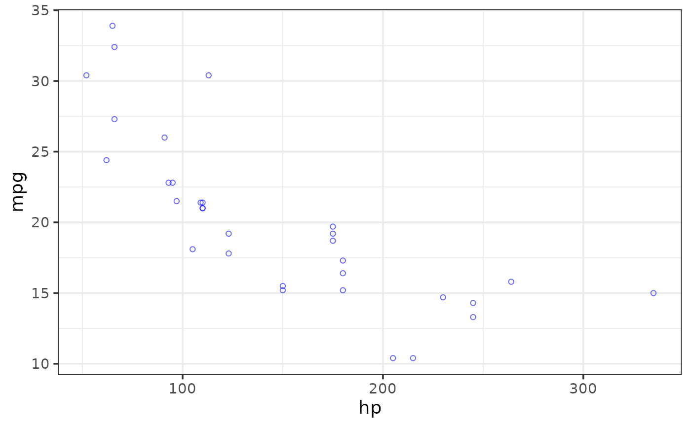
plot_scatter(mtcars, y = mpg, x = hp, colour = "blue")
 # \donttest{
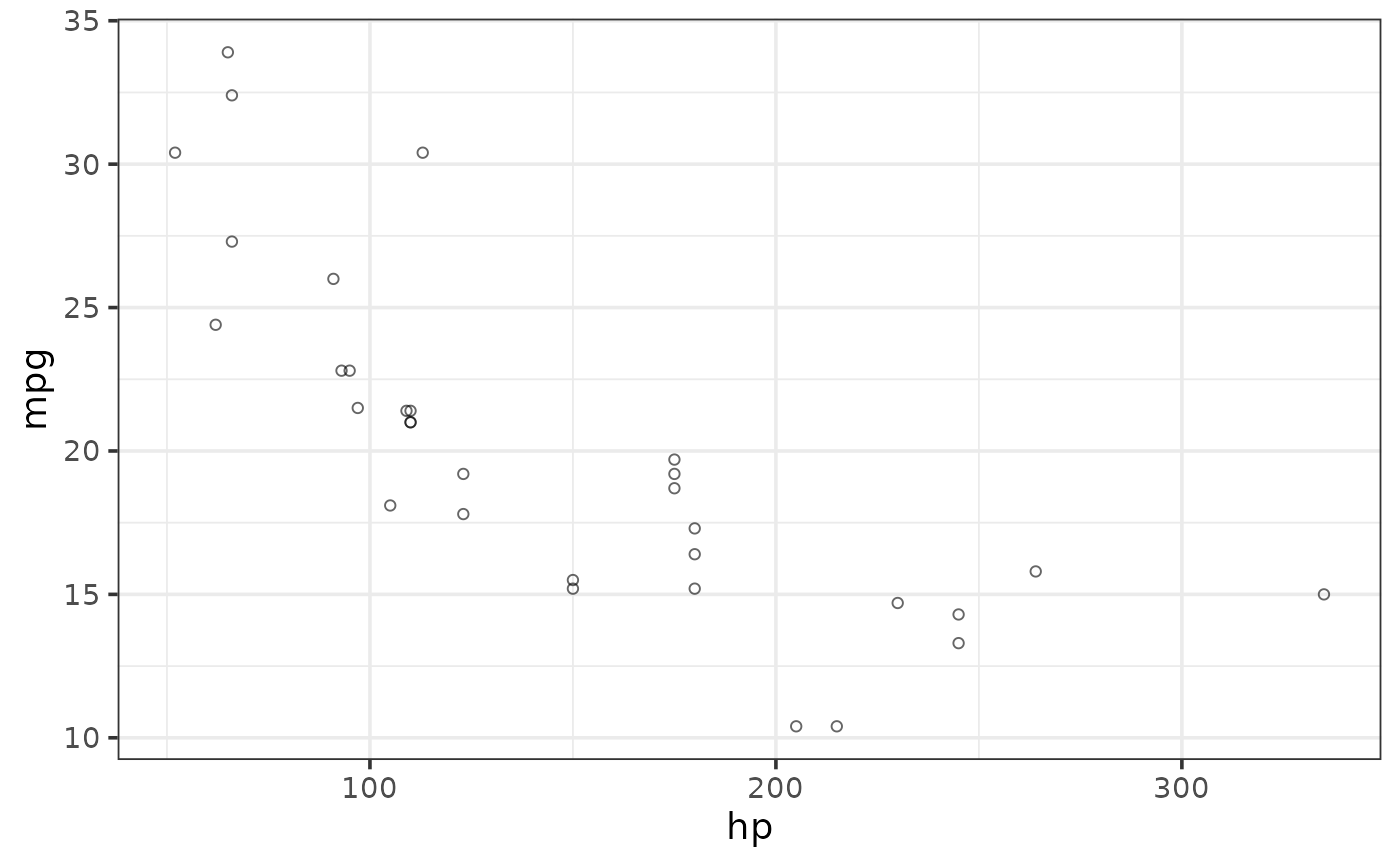
plot_scatter(mtcars, y = mpg, x = hp)
# \donttest{
plot_scatter(mtcars, y = mpg, x = hp)
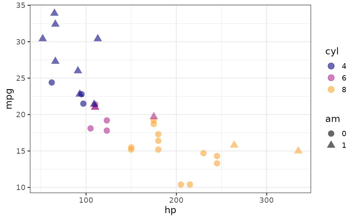
 plot_scatter(mtcars, y = mpg, x = hp,
colour_var = cyl, shape_var = am, size = 4)
plot_scatter(mtcars, y = mpg, x = hp,
colour_var = cyl, shape_var = am, size = 4)
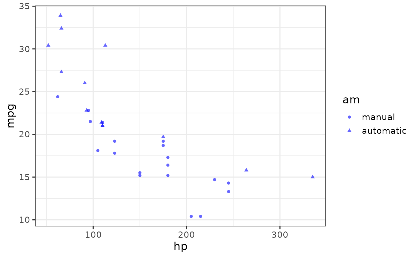
 plot_scatter(mtcars, y = mpg, x = hp, colour = "blue",
shape_var_labs = c("manual" = "0", "automatic" = "1"),
shape_var = am, theme = "bw")
plot_scatter(mtcars, y = mpg, x = hp, colour = "blue",
shape_var_labs = c("manual" = "0", "automatic" = "1"),
shape_var = am, theme = "bw")
 #map colour, shape, and size to different variables
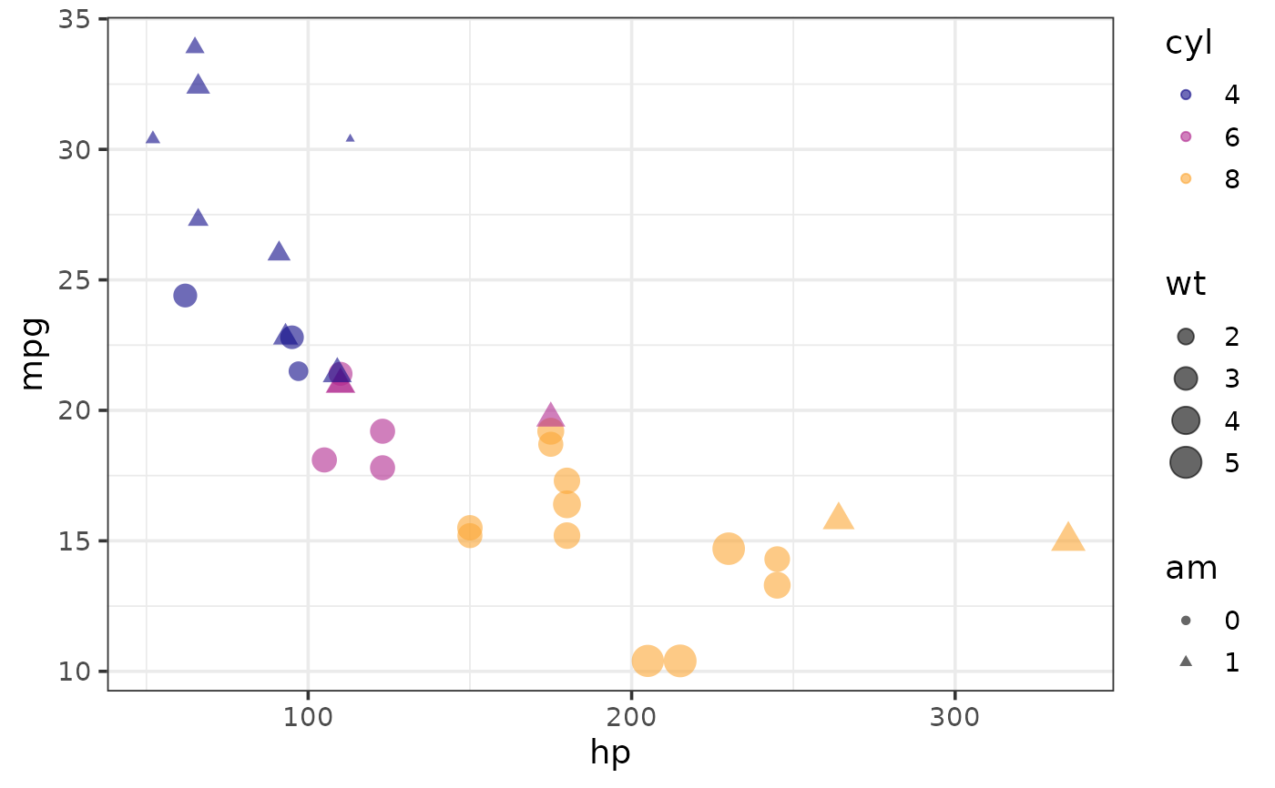
plot_scatter(mtcars, y = mpg, x = hp,
colour_var = cyl, shape_var = am, size_var = wt)
#map colour, shape, and size to different variables
plot_scatter(mtcars, y = mpg, x = hp,
colour_var = cyl, shape_var = am, size_var = wt)
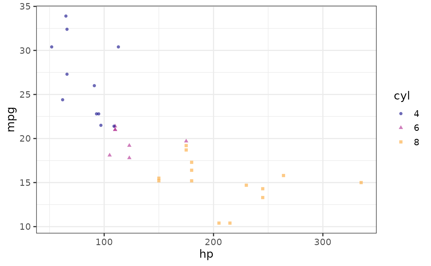
 #map colour and shape to a common variable
plot_scatter(mtcars, y = mpg, x = hp,
shape_var = cyl, colour_var = cyl)
#map colour and shape to a common variable
plot_scatter(mtcars, y = mpg, x = hp,
shape_var = cyl, colour_var = cyl)
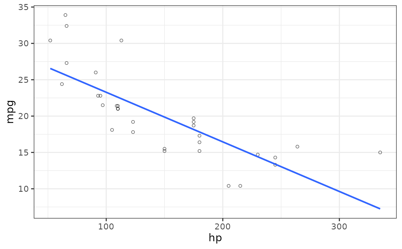
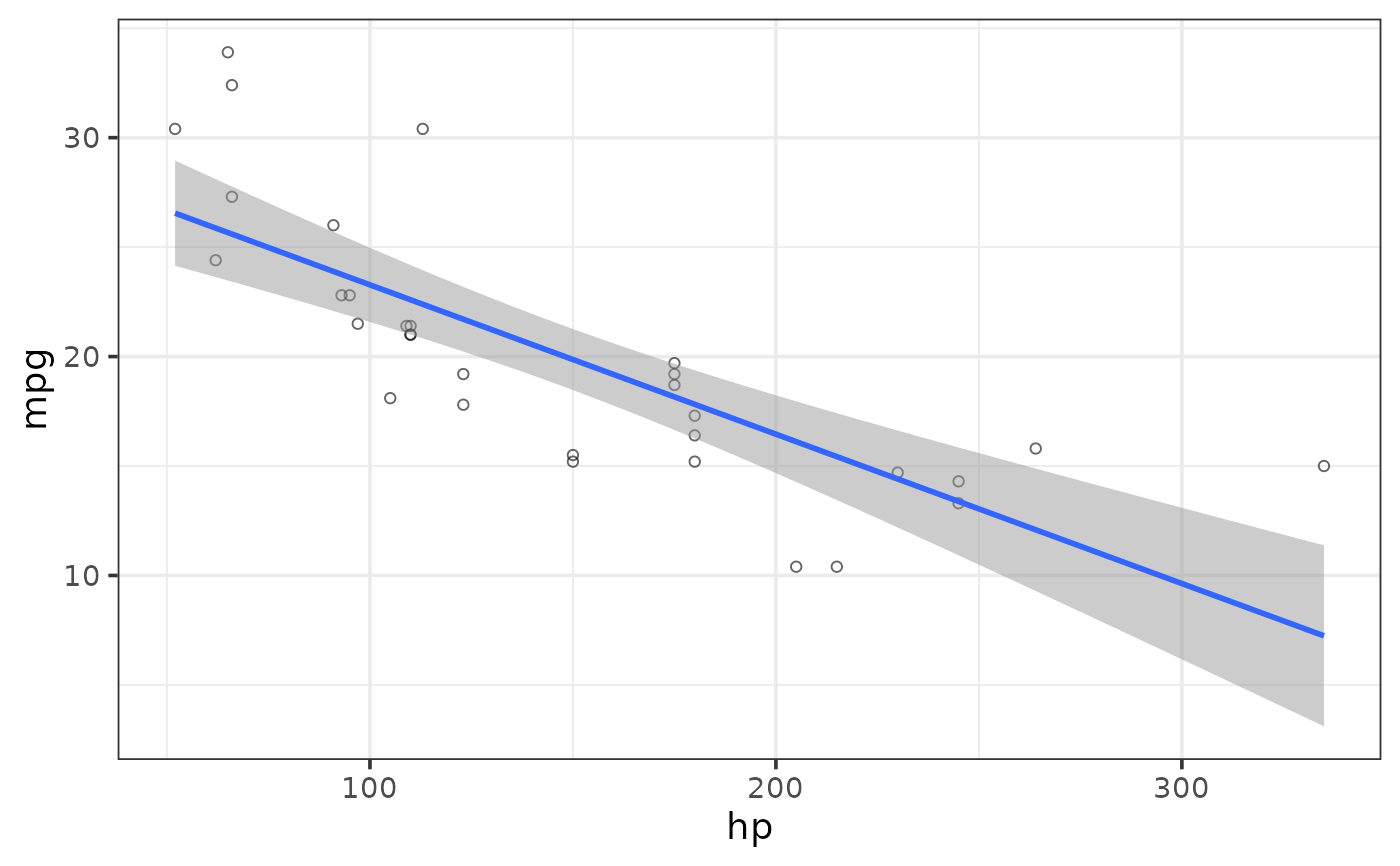
 #add a regression line
#linear
plot_scatter(mtcars, y = mpg, x = hp,
regression_line = TRUE, regression_method = "lm")
#add a regression line
#linear
plot_scatter(mtcars, y = mpg, x = hp,
regression_line = TRUE, regression_method = "lm")
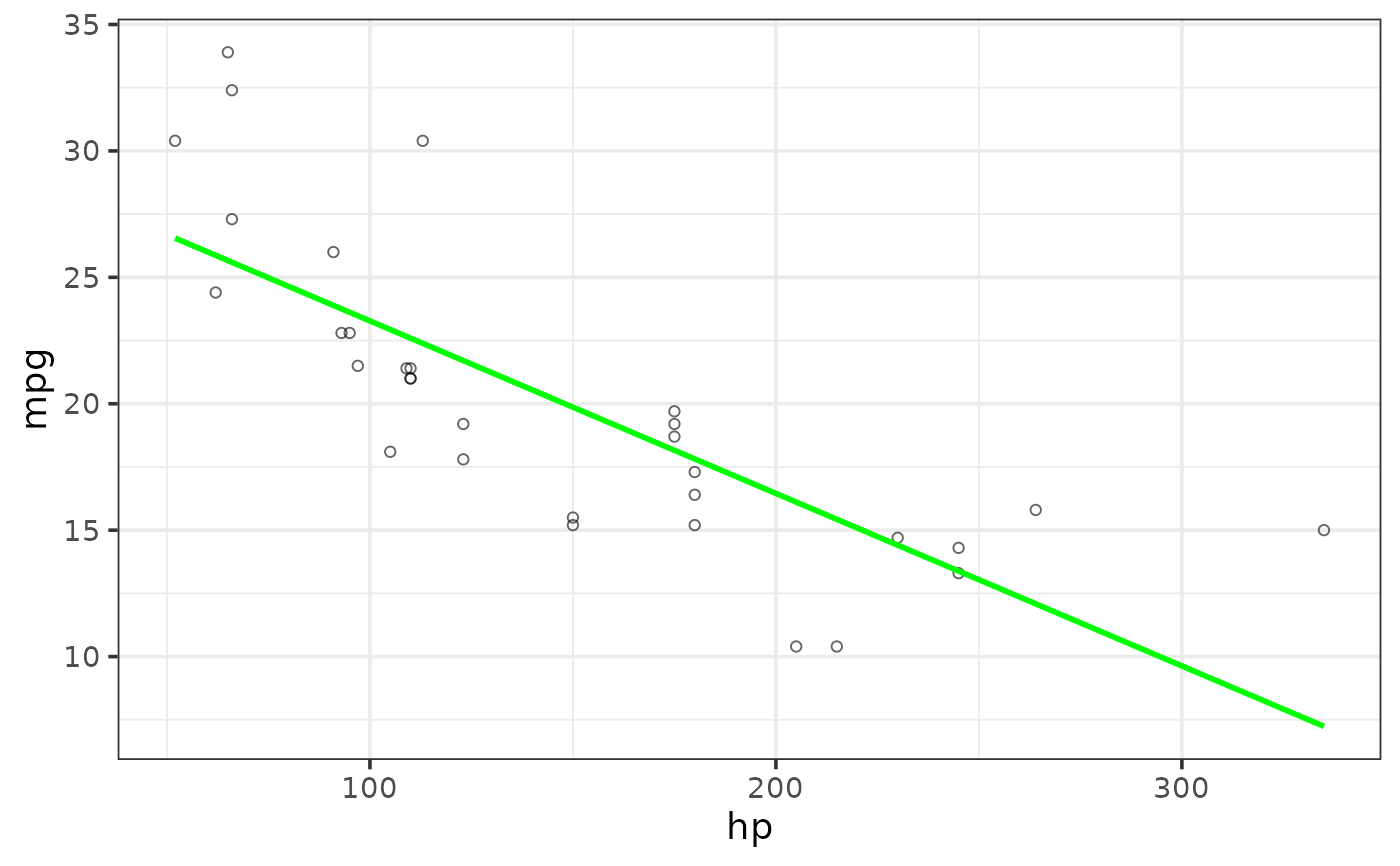
 #change the regression line colour
plot_scatter(mtcars, y = mpg, x = hp,
regression_line = TRUE, regression_method = "lm",
regression_line_colour = "green")
#change the regression line colour
plot_scatter(mtcars, y = mpg, x = hp,
regression_line = TRUE, regression_method = "lm",
regression_line_colour = "green")
 #add standard error envelope
plot_scatter(mtcars, y = mpg, x = hp,
regression_line = TRUE, regression_method = "lm",
regression_se = TRUE)
#add standard error envelope
plot_scatter(mtcars, y = mpg, x = hp,
regression_line = TRUE, regression_method = "lm",
regression_se = TRUE)
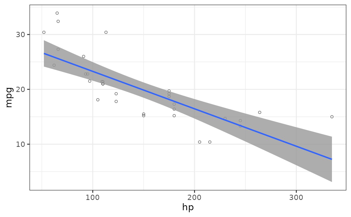
 #adjust standard error envelope transparency
plot_scatter(mtcars, y = mpg, x = hp,
regression_line = TRUE, regression_method = "lm",
regression_se = TRUE,
regression_alpha = 0.8) #default is 0.5
#adjust standard error envelope transparency
plot_scatter(mtcars, y = mpg, x = hp,
regression_line = TRUE, regression_method = "lm",
regression_se = TRUE,
regression_alpha = 0.8) #default is 0.5
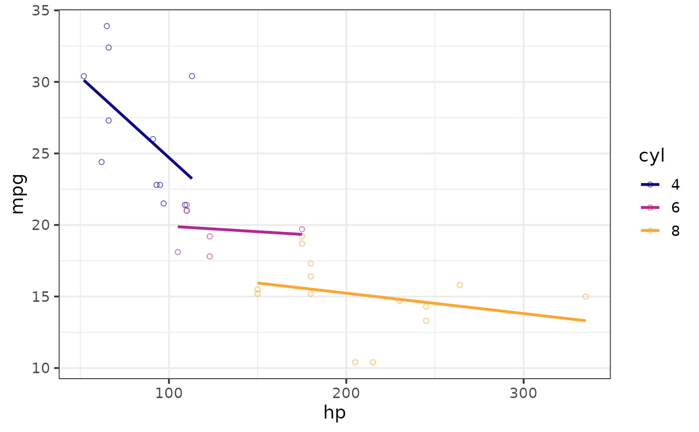
 #split by a grouping variable
plot_scatter(mtcars, y = mpg, x = hp, colour_var = cyl,
regression_line = TRUE, regression_method = "lm")
#split by a grouping variable
plot_scatter(mtcars, y = mpg, x = hp, colour_var = cyl,
regression_line = TRUE, regression_method = "lm")
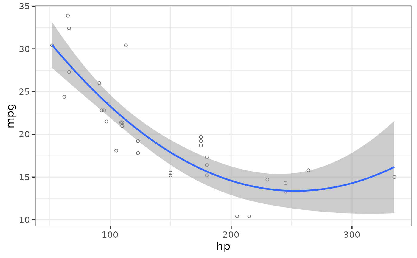
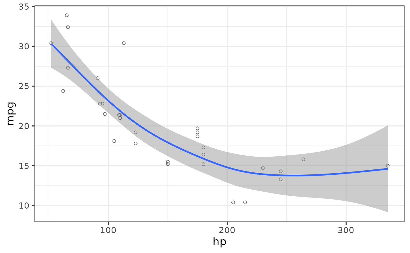
 #fit a polynomial regression line by specifying a regression_formula = formula()
plot_scatter(mtcars, y = mpg, x = hp,
regression_line = TRUE, regression_method = "lm", regression_se = TRUE,
regression_formula = y ~ poly(x, 2))
#fit a polynomial regression line by specifying a regression_formula = formula()
plot_scatter(mtcars, y = mpg, x = hp,
regression_line = TRUE, regression_method = "lm", regression_se = TRUE,
regression_formula = y ~ poly(x, 2))
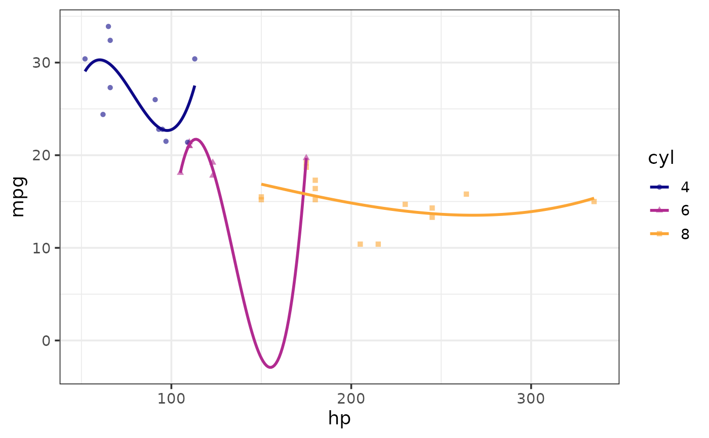
 plot_scatter(mtcars, y = mpg, x = hp, shape_var = cyl, colour_var = cyl,
regression_line = TRUE, regression_method = "lm",
regression_formula = y ~ poly(x, 3))
plot_scatter(mtcars, y = mpg, x = hp, shape_var = cyl, colour_var = cyl,
regression_line = TRUE, regression_method = "lm",
regression_formula = y ~ poly(x, 3))
 #fit a non-linear regression line using locally(-weighted) scatterplot smoothing (loess)
plot_scatter(mtcars, y = mpg, x = hp,
regression_line = TRUE, regression_se = TRUE,
regression_method = "loess")
#fit a non-linear regression line using locally(-weighted) scatterplot smoothing (loess)
plot_scatter(mtcars, y = mpg, x = hp,
regression_line = TRUE, regression_se = TRUE,
regression_method = "loess")
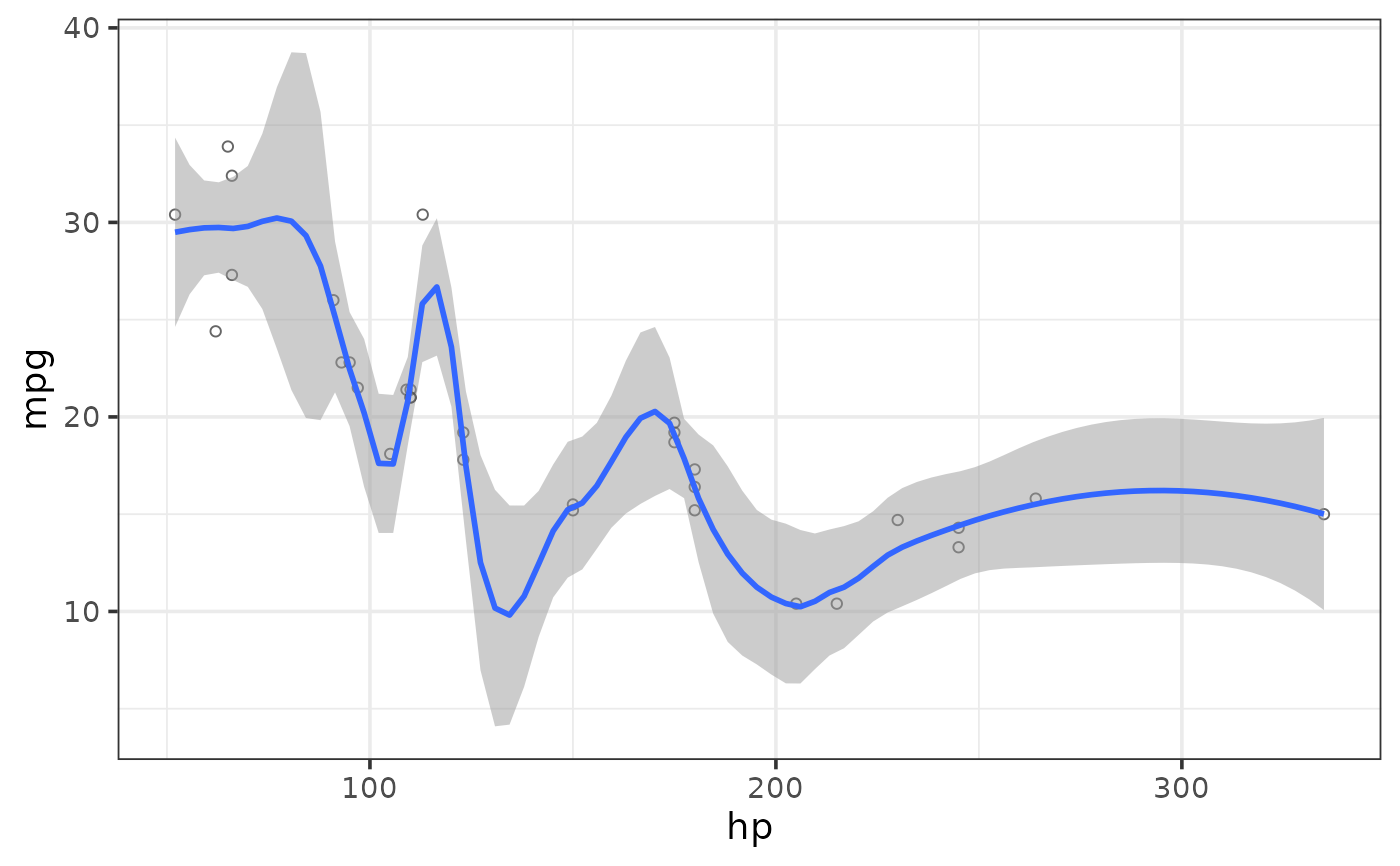
 #fit a non-linear regression line using locally(-weighted) scatterplot smoothing (loess)
#& also adjust the span (default = 0.75).
#This controls how much of the data is used for the weighted smoothing.
plot_scatter(mtcars, y = mpg, x = hp,
regression_line = TRUE, regression_se = TRUE,
regression_method = "loess", loess_span = 0.3)
#fit a non-linear regression line using locally(-weighted) scatterplot smoothing (loess)
#& also adjust the span (default = 0.75).
#This controls how much of the data is used for the weighted smoothing.
plot_scatter(mtcars, y = mpg, x = hp,
regression_line = TRUE, regression_se = TRUE,
regression_method = "loess", loess_span = 0.3)
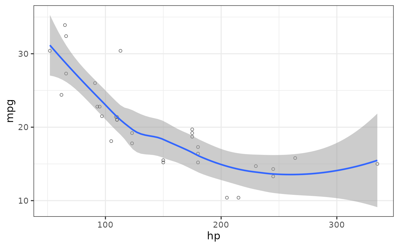
 #fit a non-linear regression line using a generalized additive model (gam), the default
plot_scatter(mtcars, y = mpg, x = hp,
regression_line = TRUE, regression_se = TRUE,
regression_method = "gam")
#fit a non-linear regression line using a generalized additive model (gam), the default
plot_scatter(mtcars, y = mpg, x = hp,
regression_line = TRUE, regression_se = TRUE,
regression_method = "gam")
 #use a dashed regression line instead
plot_scatter(mtcars, y = mpg, x = hp,
regression_line = TRUE, regression_se = TRUE, regression_line_type = "dashed")
#use a dashed regression line instead
plot_scatter(mtcars, y = mpg, x = hp,
regression_line = TRUE, regression_se = TRUE, regression_line_type = "dashed")
 #more complex example with overplotting
plot_scatter(pdata, y = y1, x = d, colour_var = g,
regression_line = TRUE)
#more complex example with overplotting
plot_scatter(pdata, y = y1, x = d, colour_var = g,
regression_line = TRUE)
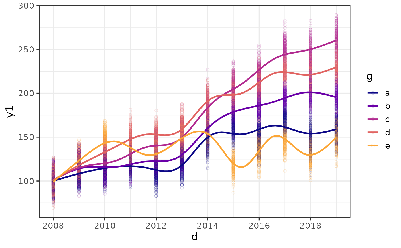
 #option 1 for dealing with overplotting: add jittering to offset overlappping points
plot_scatter(pdata, y = y1, x = d, colour_var = g,
jitter = TRUE,
regression_line = TRUE)
#option 1 for dealing with overplotting: add jittering to offset overlappping points
plot_scatter(pdata, y = y1, x = d, colour_var = g,
jitter = TRUE,
regression_line = TRUE)
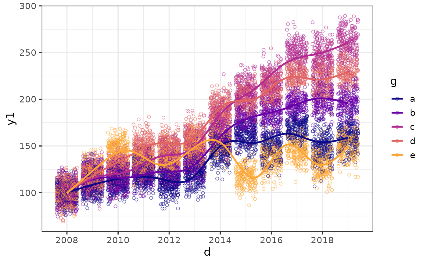 #option 2: make overlapping values more transparent
plot_scatter(pdata, y = y1, x = d, colour_var = g,
alpha = 0.2,
regression_line = TRUE)
#option 2: make overlapping values more transparent
plot_scatter(pdata, y = y1, x = d, colour_var = g,
alpha = 0.2,
regression_line = TRUE)
 #option 3: do both and make it interactive
plot_scatter(pdata, y = y1, x = d, colour_var = g,
jitter = TRUE, alpha = 0.2,
regression_line = TRUE, interactive = TRUE)
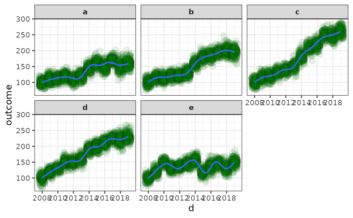
#add a faceting variable
plot_scatter(pdata, y = y1, x = d,
colour = "black", shape = 21, fill = "green4",
jitter = TRUE, size = 4, alpha = 0.1,
regression_line = TRUE, regression_se = TRUE,
facet_var = g,
ylab = "outcome",
theme = "bw")
#option 3: do both and make it interactive
plot_scatter(pdata, y = y1, x = d, colour_var = g,
jitter = TRUE, alpha = 0.2,
regression_line = TRUE, interactive = TRUE)
#add a faceting variable
plot_scatter(pdata, y = y1, x = d,
colour = "black", shape = 21, fill = "green4",
jitter = TRUE, size = 4, alpha = 0.1,
regression_line = TRUE, regression_se = TRUE,
facet_var = g,
ylab = "outcome",
theme = "bw")
 # }
# }